Welcome back to the deep learning & medical image analysis course. Today we are finally breaking away from classification. We will be learning all about one of the most widely used tasks in medical image analysis: Image Segmentation. Ironically, it is very similar to classification, just at a far more granular (pixel-level) scale. We will start by defining what segmentation is and what the most common types of segmentation are. Then we will dive into foundational deep-learning (specifically convolutional neural network) based segmentation methods.
The next piece of the puzzle that we will discuss are the loss functions (some of which we have seen before!) that are used for image segmentation. Then we will shift into medical image segmentation and take a deep dive into a frequently used neural network architecture for medical segmentation: U-Net and it's variants.
After selecting an architecture and the loss functions, the next thing that you want to decide on is the way you input data. Frequently (in histopathalogy, MRI, or CT) images are simply too big to fit into your model in one go. There are different methods to deal with this limitation. Simultaneously, we will also discuss how to properly augment the data for each case. Next, we will briefly discuss how to improve segmentation of small objects. Then we will shift our focus various inference and post-processing techniques to improve performance when we deploy the model.
We will finish our tutorial by discussing a common benchmark method: nnUNet. We will discuss its benefits and its limitations. Finally, we discuss the Segment Anything Model (SAM) and some of its medically oriented variants.
Important notes
- It is fine to consult with colleagues to solve the problems, in fact it is encouraged.
- Please turn off AI tools, we want you to memorize concepts and not just quickly breeze through problems. To turn off AI click on the gear in the top right corner. got to AI assistance -> Untick Show AI powered inline completions, Untick consented to use generative AI features, tick Hide Generative AI features
8 Medical Image Segmentation using Convolutional Neural Networks
8.1 Environment Setup
Running the cells below will set up your environment on either your local (Windows) computer or on Google Colab.
You will also be given a zipped up data file. Put it into your environment and unpack it (directly if you are running it locally, upload it to the google colab files if you are in google colab, this will take a few minutes to upload).
Be mindful of the path to the data that this creates if in the data folder there is another folder called data, then you should move that folder to the root! Otherwise you will have import errors later!
You can download it here:
# Detect environment (Colab vs Local)
import sys
import os
import shutil
import stat

IN_COLAB = 'google.colab' in sys.modules

# GitHub repository configuration
GITHUB_USER = "RiaanZoetmulder"
GITHUB_REPO = "deep_learning_course"
GITHUB_BRANCH = "main"

if IN_COLAB:
    print("Running in Google Colab")
    WORKING_DIR = "/content"
else:
    print("Running locally")
    WORKING_DIR = os.getcwd()

# Temporary clone location
REPO_DIR = os.path.join(WORKING_DIR, GITHUB_REPO)

# Target directories in working directory
SESSION_DIR = os.path.join(WORKING_DIR, 'session_008')
MEDIA_DIR = os.path.join(WORKING_DIR, 'media')
HELPERS_DIR = os.path.join(WORKING_DIR, 'general_helpers')

def force_remove_readonly(func, path, excinfo):
    """Handle Windows read-only files during shutil.rmtree"""
    os.chmod(path, stat.S_IWRITE)
    func(path)

# Clone repo and extract needed folders
if not os.path.exists(SESSION_DIR) or not os.path.exists(HELPERS_DIR):
    # Clone if not already cloned
    if not os.path.exists(REPO_DIR):
        !git clone https://github.com/{GITHUB_USER}/{GITHUB_REPO}.git {REPO_DIR}
        print(f"✓ Cloned {GITHUB_REPO}")

    # Copy lecture_6/session_008 → session_008
    if not os.path.exists(SESSION_DIR):
        shutil.copytree(os.path.join(REPO_DIR, 'lecture_6', 'session_008'), SESSION_DIR)
        print(f"✓ Copied session_008")

    # Copy lecture_6/media → media
    if not os.path.exists(MEDIA_DIR):
        shutil.copytree(os.path.join(REPO_DIR, 'lecture_6', 'media'), MEDIA_DIR)
        print(f"✓ Copied media")

    # Copy general_helpers → general_helpers
    if not os.path.exists(HELPERS_DIR):
        shutil.copytree(os.path.join(REPO_DIR, 'general_helpers'), HELPERS_DIR)
        print(f"✓ Copied general_helpers")

    # Clean up cloned repo (with Windows read-only file handling)
    shutil.rmtree(REPO_DIR, onerror=force_remove_readonly)
    print(f"✓ Cleaned up temporary clone")
else:
    print("✓ Code folders already exist")

# Add module paths
sys.path.insert(0, SESSION_DIR)
sys.path.insert(0, HELPERS_DIR)

print(f"Module paths configured for {'Colab' if IN_COLAB else 'local'} environment")


MEDIA_FOLDER_PARTS = ["media"]  # OS-agnostic path components

# Set up local media path based on environment (OS-agnostic)
if IN_COLAB:
    MEDIA_ROOT = os.path.join("/content", *MEDIA_FOLDER_PARTS)
else:
    MEDIA_ROOT = os.path.join(".", *MEDIA_FOLDER_PARTS)

print('Set up Media Root folder at: ', MEDIA_ROOT)
import sys
import os
import subprocess

# Check if we're in a virtual environment
IN_VENV = sys.prefix != sys.base_prefix
VENV_PATH = os.path.join(os.getcwd(), '.venv')

if not IN_VENV and not IN_COLAB:
    print("=" * 70)
    print("⚠️  NOT RUNNING IN A VIRTUAL ENVIRONMENT")
    print("=" * 70)
    print("\nFollow these steps to set up your environment:\n")
    print("1. Open a terminal in VSCode (Ctrl+` or Terminal > New Terminal)")
    print("2. Run these commands:\n")
    print(f'   python -m venv .venv')
    print(f'   .venv\\Scripts\\activate')
    print(f'   pip install ipykernel --index-url https://pypi.org/simple/')
    print(f'   python -m ipykernel install --user --name=deep_learning_course --display-name="Deep Learning Course"')
    print("\n3. In VSCode, click 'Select Kernel' (top right of notebook)")
    print("4. Choose 'Python Environments...' > '.venv (Python x.x.x)'")
    print("   OR choose 'Jupyter Kernel...' > 'Deep Learning Course'")
    print("\n5. Re-run this cell to install packages (I've had to restart the kernel, the notebook, or even VSCode after setting up the venv for it to recognize the new environment)")
    print('NOTE: Installation of the required packages takes about 4 minutes on my machine. Please be patient and wait for the "Environment ready!" message before running the rest of the notebook \n or smashing your computer in frustration.')
    print("=" * 70)

elif IN_VENV or IN_COLAB:
    print(f"✓ Running in virtual environment: {sys.prefix}")
    print(f"✓ Python executable: {sys.executable}")
    print("\nInstalling required packages...")

    # Install packages using subprocess to ensure we use the right pip
    packages = [
        "ipykernel",
        "scikit-learn",
        "opencv-python",
        "pydicom",
        "ipywidgets",
        "numpy",
        "matplotlib"
    ]

    # Install base packages
    subprocess.run([
        sys.executable, "-m", "pip", "install", "-q",
        "--index-url", "https://pypi.org/simple/",
        *packages
    ], capture_output=True, text=True)
    print("✓ Base packages installed")

    # Install PyTorch (separate due to size)
    subprocess.run([
        sys.executable, "-m", "pip", "install", "-q",
        "--index-url", "https://pypi.org/simple/",
        "torch", "torchvision"
    ], capture_output=True, text=True)
    print("✓ PyTorch installed")

    # Register kernel if not already registered
    subprocess.run([
        sys.executable, "-m", "ipykernel", "install",
        "--user", "--name=deep_learning_course",
        "--display-name=Deep Learning Course"
    ], capture_output=True, text=True)
    print("✓ Jupyter kernel registered")

    print("\n" + "=" * 70)
    print("✓ Environment ready! You can now run the rest of the notebook.")
    print("=" * 70)
# NOTE: After uploading data.zip, run this when in colab
# Make sure you upload the data zip file to google colab first.
if IN_COLAB:
  !unzip data.zip -d /content/
# Core imports

# HINT: If you have a module not found error, you have to rerun the first code cell in this notebook
# It adds all the paths to sys, such that custom modules are found.
import sys
import os
import torch
import torch.nn as nn
import torch.nn.functional as F
import torchvision
from typing import List, Tuple
from torchvision import transforms
import pydicom as pdm

import numpy as np
import matplotlib.pyplot as plt

# custom imports
from ct_visualization import load_dicom_series, show_normalization_comparison, create_normalization_slider
from display_media import show_figure, show_video
from github_assets import download_media_assets
from feature_extraction import extract_vgg_features
from video_segmentation import display_video_segmentation

# Set device
device = torch.device('cuda' if torch.cuda.is_available() else 'cpu')
print(f"Using device: {device}")
8.2 What is segmentation
When we are classifying our goal is to know what object is on the image, when we are segmenting we want to know what an object is and what pixels belong to the object on the image. We are interested in image segmentation for several reasons:
- We would like to know where on an image a certain object is located. Segmentation will give you fine-grained information about the object location in the image.
- We would like to know the exact borders of an object in an image. This can be useful information on its own, but in medical image analysis it can also be an important preliminary step in order to quantify features (such as texture, intensity, volume etc.) of the underlying object in the image. A reason why you would be interested in segmentation-mask derived features is because they can inform clinical measures such as treatment outcome or prognosis.
- We would like to know the count of objects in an image.
An example in medical image analysis could be Multiple-sclerosis (MS) lesion segmentation. MS lesions are a type of lesion that are visible on MRI scans in the white matter of the brain. They indicate that certain axons in the brain have been demyelinated. Not only is the volume important clinically, but also the location of the lesions, and also the count. The downside of segmentation is that it is very labor intensive to annotate. An example from my own work is the segmentation of brain tissue types on MRI scans of newborn babies. To annotate a single MRI volume could easily take more than an entire working week for a medical professional. The lesson from this is that you should first consider creating other types of annotations for other types of tasks than segmentation if you are interest in only location data or count.
One type of task that we will cover a few lectures later is object detection. In an object detection setting all you need to know are the coordinates of a box that bounds the object of interest (called a bounding box). In the image below you can see the difference in how these tasks end up looking and what their target labels look like.
show_figure("classification_detection_segmentation_comparison.png", width = 1500, media_root = MEDIA_ROOT)

mssg = """
---- NOTE ----
Bear in mind that in NumPy (which we are using to plot the images), the convention for coordinates is (row, column) which corresponds to (y, x) in Cartesian coordinates.\n This can lead to confusion when interpreting the axes of the images, especially for those familiar with the (x, y) convention in Cartesian space.\n
Moreover, the coordinates in the images are often displayed with the origin (0, 0) at the top-left corner. So be careful when intereting the bounding box label.
\n
The segmentation label example is derived from the real segmentation max, but downsampled used nearest neighbour interpolation. The real label has the same resolution as the original image.
"""
print(mssg)
Like there are different types of classification (binary, multi-class, multi-label etc.) there are also multiple types of segmentation task. Here we will briefly describe two.
8.2.1 Semantic Segmentation
Semantic segmentation answers the question: “what class is each pixel?” Instead of predicting one label for the whole image (classification), the model outputs a 2D label map with the same width and height as the input image, where each pixel stores a class ID (e.g., background, lesion, organ). A key detail is that semantic segmentation does not distinguish between different objects of the same class: if there are three lesions (or three cars in Pascal VOC), all those pixels are labeled as the same class.
8.2.2 Instance Segmentation
Instance segmentation answers the question: “which pixels belong to which individual object?” It still produces pixel-level masks, but now it separates different objects even if they share the same class (lesion A vs lesion B). You can think of the label as a list of instances, where each instance has a class label and its own binary mask (or an instance ID image where each object gets a unique ID). This is useful when you care about counting objects and measuring properties per object (e.g., lesion count and per-lesion volume).
Examples are shown below.
show_figure("semantic_vs_instance_comparison.png", width = 1500, media_root = MEDIA_ROOT)
8.3 Foundational Deep Learning Segmentation Methods
So far we have learned about classification. If we wanted to segment an image, one way in which we could do that is by sliding a simple convolutional neural network that is trained to segment pixels over each image that we wanted to segment. In fact, this is how many pre-deep learning (and some early deep learning based segmentation methods) worked. The downside of doing this is that it is computationally very expensive and you limit your receptive field.
Ideally, we would input the entire image into the neural network and predict the entire segmentation mask in one time. So we would like to have some way of inverting a convolution operation, where at each step we up-sample our feature map back to the image dimensions with an arbitrary number of channels (each channel corresponding to a specific class).
Fortunately, there is an operation that approximates exactly that: The Transposed Convolution.
8.3.1 The Transposed Convolution
In the previous lectures we have learned about regular convolutionals. These convolutions slide a learnable kernel over input images. After each convolutional layer, the size of the input stays the same or it is downsampled. When we talk about segmentation, we would really like to revert these operations such that we end up with an output that has the same height and width as the input image. This would allow us to predict the entire segmentation map in one pass (or do cool generative AI things, but that's for another day!).
One of the operations that is used to learn how to invert a regular convolution is called a transposed convolution (also often referred to as a fractionally strided convolution, up-convolution or a deconvolution, though the latter is not technically correct). The transposed convolution works as follows. You take an input and in between the elements you insert a constant value. Additionally, you add zero padding around this new interlaced input. Then you convolve it with a learnable kernel, just like a regular convolution. The end result is an operation that approximates the inverse of a convolution operation. See the video below for how this works!
show_video("transposed_conv_2d.mp4", width = 900, media_root = MEDIA_ROOT)
Calculating the Output Size of a Transposed Convolution
For a regular convolution, the output size shrinks (or stays the same with padding). For a transposed convolution, the output size grows.
Recall the steps:
- Interlace: Insert
stride - 1(or more) zeros between each input element - Pad: Add
paddingzeros around the interlaced input - Convolve: Apply a regular convolution with the kernel
The formula to calculate the output size is:
$$H_{out} = (H_{in} - 1) \times \text{stride} + 2 \times \text{padding} - (\text{kernel\_size} - 1) + 1$$Which simplifies to:
$$H_{out} = (H_{in} - 1) \times \text{stride} + 2 \times \text{padding} - \text{kernel\_size} + 2$$Example: If you have a 5×5 input, a 3×3 kernel, stride=2, and padding=0: $$H_{out} = (5 - 1) \times 2 + 0 - 3 + 2 = 8 - 1 = 7$$
So a 5×5 input becomes a 7×7 output (matching what the animation showed).
There are two additional parameters rarely used in practice:
- dilation: spacing between kernel elements (default 1)
- output_padding: extra padding added to the output after convolution
The full formula becomes:
$$H_{out} = (H_{in} - 1) \times \text{stride} + 2 \times \text{padding} - \text{dilation} \times (\text{kernel\_size} - 1) + \text{output\_padding} + 1$$PyTorch Implementation Note: In torch.nn.ConvTranspose2d, the padding parameter is inverted compared to the mathematical definition above. PyTorch specifies how much to subtract from the maximum possible padding:
This transforms our formula into PyTorch's version:
$$H_{out} = (H_{in} - 1) \times \text{stride} - 2 \times \text{padding} + \text{dilation} \times (\text{kernel\_size} - 1) + \text{output\_padding} + 1$$Why is the definition in PyTorch slightly different from regular one?
They differ to make implementation of certain network architectures easier. Recall that a transposed convolution is used to invert a regular convolution. By setting padding parameter of Conv2d and ConvTranspose2d to be each others inverse, it allows you to keep things consistent.
Let's look at an example
# Example input tensor
input_tensor = torch.randn(1, 256, 8, 8)

print('Input tensor shape:', input_tensor.shape)

class TransposedConv2dExample(nn.Module):
    def __init__(self, in_channels: int=256, out_channels:int =128, kernel_size:int=3, stride:int=2, padding:int=1, output_padding:int=1):
        super(TransposedConv2dExample, self).__init__()
        """
        Single Layer Transpose Convolutional Network

        Bit superfluous to put it into an nn.Module. But we do want to reinforce the habit of using them :)
        """
        self.transposed_conv = nn.ConvTranspose2d(
            in_channels, out_channels, kernel_size, stride, padding, output_padding
        )

    def forward(self, x):
        return self.transposed_conv(x)

# Create an instance of the model and move it to the appropriate device
model = TransposedConv2dExample().to(device)

output_tensor = model(input_tensor.to(device))

print('Output tensor shape:', output_tensor.shape)
A more realistic example: The Upsampling Path
This is a simple example of upsampling a tensor of size [1, 256, 8, 8] to [1, 128, 16, 16]. However, much like regular convolutional neural networks we can repeatedly upsample until we reach the desired shape. In the example below I will show you how to do this more realistically, adding different operations that you would add in a real network as well.
# the Input tensor, we are starting with a lot of channels, but very low height and width.
# This is a common scenario in the decoder part of a segmentation model,
# where we have a feature map with many channels (representing different features) but low spatial resolution (height and width).
input_tensor = torch.randn(1, 1024, 4, 4)

print('RECALL: The Dimensions are: (batch_size, channels, height, width)')
print('Input tensor shape:', input_tensor.shape)

class ExampleUpsamplingLayer(nn.Module):
    def __init__(
            self,
            in_channels: int=1024,
            out_channels:int=512,
            kernel_size:int=3,
            stride:int=2,
            padding:int=1,
            output_padding:int=1) -> None:
        super(ExampleUpsamplingLayer, self).__init__()
        """
        Example Upsampling Layer using Transposed Convolution

        Simple: transposed_convolution -> batch normalization -> ReLU
        """
        self.transposed_conv = nn.ConvTranspose2d(
            in_channels, out_channels, kernel_size, stride, padding, output_padding
        )

        self.relu = nn.ReLU()
        self.batch_norm = nn.BatchNorm2d(out_channels)  # Batch normalization

    def forward(self, x):
        x = self.transposed_conv(x)
        x = self.batch_norm(x)
        x = self.relu(x)
        return x


class ExampleUpsamplingModule(nn.Module):
    def __init__(self, in_channels: int=1024) -> None:
        super(ExampleUpsamplingModule, self).__init__()
        """
        Example Upsampling Module using Transposed Convolution

        We will create a simple upsampling module that takes an input tensor with 1024 channels and spatial dimension of 4.
        The module will use 6 layers of transposed convolutions to upsample the feature map to a spatial dimension of 256x256.

        The final layer will be a regular convolutional layer, which keeps the spatial dimensions the same but reduces the number of target channels.
        In case of binary segmentation (background vs foreground), this would just be the assignment of probability values to each pixels.
        """

        ## LAYER 1 - Upsampling from 1024 channels to 512 channels, and doubling the spatial dimensions to 8x8
        self.upsample1 = ExampleUpsamplingLayer(
            in_channels=in_channels,
            out_channels=512,
            kernel_size=3,
            stride=2,
            padding=1,
            output_padding=1
        )

        ## LAYER 2 - Upsampling from 512 channels to 256 channels, and doubling the spatial dimensions to 16x16
        self.upsample2 = ExampleUpsamplingLayer(
            in_channels=512,
            out_channels=256,
            kernel_size=3,
            stride=2,
            padding=1,
            output_padding=1
        )

        ## LAYER 3 - Upsampling from 256 channels to 128 channels, and doubling the spatial dimensions to 32x32
        self.upsample3 = ExampleUpsamplingLayer(
            in_channels=256,
            out_channels=128,
            kernel_size=3,
            stride=2,
            padding=1,
            output_padding=1
        )

        ## LAYER 4 - Upsampling from 128 channels to 64 channels, and doubling the spatial dimensions to 64x64
        self.upsample4 = ExampleUpsamplingLayer(
            in_channels=128,
            out_channels=64,
            kernel_size=3,
            stride=2,
            padding=1,
            output_padding=1
        )

        ## LAYER 5 - Upsampling from 64 channels to 32 channels, and doubling the spatial dimensions to 128x128
        self.upsample5 = ExampleUpsamplingLayer(
            in_channels=64,
            out_channels=32,
            kernel_size=3,
            stride=2,
            padding=1,
            output_padding=1
        )

        ## LAYER 6 - Upsampling from 32 channels to 16 channels, and doubling the spatial dimensions to 256x256
        self.upsample6 = ExampleUpsamplingLayer(
            in_channels=32,
            out_channels=16,
            kernel_size=3,
            stride=2,
            padding=1,
            output_padding=1
        )

        ## Out Layer - Final convolution to get the desired number of output channels (e.g., 1 for binary segmentation)
        # NOTE: Do not add an activation here, we would have to pass it to the loss function
        # (e.g., BCEWithLogitsLoss) which expects raw logits.
        self.out_layer = nn.Conv2d(16, 1, kernel_size=1)

    def forward(self, x: torch.Tensor) -> torch.Tensor:
        x = self.upsample1(x)
        x = self.upsample2(x)
        x = self.upsample3(x)
        x = self.upsample4(x)
        x = self.upsample5(x)
        x = self.upsample6(x)
        x = self.out_layer(x)
        return x

# Create an instance of the upsampling module and move it to the appropriate device
upsampling_module = ExampleUpsamplingModule().to(device)

# Pass the input tensor through the upsampling module
output_tensor = upsampling_module(input_tensor.to(device))


print('\nOutput tensor shape:', output_tensor.shape)
This concludes our discussion of the transposed convolution, one of the earliest ways of learning how to reverse the convolution operation. One of the downsides of transposed convolutions is that they are computationally expensive (and in the case of generative AI can cause checkerboard artefacts).
More modern networks exist to that have different ways of learning how to invert a convolution. Another way for example, is to upsample using bilinear interpolation and then add a normal convolution operation. The nice thing about this is that you can play around with ways to make the regular convolution operation more efficient (such as depthwise separable convolutions that we discussed in the last lecture). We will not discuss these methods because it is beyond the scope of this lecture, but knowing they exist is important.
8.3.2 Fully Convolutional Networks (FCN)
In the previous section, you were introduced to one of the key building blocks of neural network architectures that are specifically used to segment images: The Transposed convolution. Now we are going to put that new knowledge into practice and discuss one of the earliest deep learning segmentation methods: The Fully Convolutional Network (FCN) (Long et al., 2015).
If you recall from last class, a regular convolutional neural network that we use for classification tasks will downsample images' spatial resolution, increase their number of channels, and then attach a fully connected layer to make predictions. We have already outlined a way to use this for segmentation by sliding it over an image and classifying each pixel. The problem is that this is wildly inefficient and limits you to the receptive field of the neural network.
The key insight of FCN was to remove the fully connected layers entirely and replace them with convolutional layers. This allows the network to:
- Accept images of any size (not just fixed dimensions)
- Produce spatial output maps instead of a single class prediction
FCN Architecture:
FCN uses a pretrained classification network (like VGG-16, GoogLeNet, or ResNet) as the backbone (encoder). The backbone is basically the part that does the downsampling and the encoding. It has two key modifications:
"Convolutionalized" FC layers: The fully connected layers are replaced with 1×1 convolutions. These preserve spatial information while still learning to classify.
Score layer + Upsampling: A 1×1 convolution produces class scores at low resolution, which are then upsampled back to the original image size.
The Problem with Naive Upsampling:
Simply upsampling 32× from the deepest features (FCN-32s) produces very coarse segmentations. FCN's second key innovation was skip connections that combine predictions from multiple scales. Think of it this way: At different layers in the encoder you have kernels that detect features at a different level of granularity (early on they detect edges and blobs, then textures, then they become more specific). What if you could add that information directly into the decoder path. This would allow the decoder to also use these features when making its predictions. These are what are referred to as skip connections. Below is a table that shows you where these skip connections go.
| Variant | Skip Connections | Upsample Factor | Output Quality |
|---|---|---|---|
| FCN-32s | None | 32× directly | Coarse |
| FCN-16s | pool4 features | 2× → 16× | Better |
| FCN-8s | pool4 + pool3 features | 2× → 2× → 8× | Finest |
These skip connections use element-wise addition to combine coarse semantic information from deep layers with fine spatial information from earlier layers.
FCN-VGG16 Full Architecture (FCN-8s variant):
| Layer | Operation | Output Size (H×W) | Channels | Notes |
|---|---|---|---|---|
| Input | — | H × W | 3 | RGB image |
| conv1 | 2× Conv 3×3 | H × W | 64 | |
| pool1 | MaxPool 2×2, stride 2 | H/2 × W/2 | 64 | ↓ 2× |
| conv2 | 2× Conv 3×3 | H/2 × W/2 | 128 | |
| pool2 | MaxPool 2×2, stride 2 | H/4 × W/4 | 128 | ↓ 4× |
| conv3 | 3× Conv 3×3 | H/4 × W/4 | 256 | |
| pool3 | MaxPool 2×2, stride 2 | H/8 × W/8 | 256 | ↓ 8× — save for skip |
| conv4 | 3× Conv 3×3 | H/8 × W/8 | 512 | |
| pool4 | MaxPool 2×2, stride 2 | H/16 × W/16 | 512 | ↓ 16× — save for skip |
| conv5 | 3× Conv 3×3 | H/16 × W/16 | 512 | |
| pool5 | MaxPool 2×2, stride 2 | H/32 × W/32 | 512 | ↓ 32× |
| fc6 | Conv 7×7 (was FC) | H/32 × W/32 | 4096 | "Convolutionalized" |
| fc7 | Conv 1×1 (was FC) | H/32 × W/32 | 4096 | "Convolutionalized" |
| score_fr | Conv 1×1 | H/32 × W/32 | num_classes | Class predictions at 1/32 |
| upsample_2x | TransposedConv 4×4, stride 2 | H/16 × W/16 | num_classes | ↑ 2× |
| score_pool4 | Conv 1×1 on pool4 | H/16 × W/16 | num_classes | Project pool4 to num_classes |
| fuse_pool4 | Element-wise add | H/16 × W/16 | num_classes | + score_pool4 |
| upsample_2x | TransposedConv 4×4, stride 2 | H/8 × W/8 | num_classes | ↑ 2× |
| score_pool3 | Conv 1×1 on pool3 | H/8 × W/8 | num_classes | Project pool3 to num_classes |
| fuse_pool3 | Element-wise add | H/8 × W/8 | num_classes | + score_pool3 |
| upsample_8x | TransposedConv 16×16, stride 8 | H × W | num_classes | ↑ 8× — final output |
"""
IMPORTANT NOTE

First we will show how to implement VGG! This is quite instructive
because it's been a while since we have implemented a convolutional neural network,
and it will be good to have a refresher on how to do that.
"""


class VGGConvolutionalBlock(nn.Module):
    def __init__(self, in_channels: int, out_channels: int, blocks: int = 2) -> None:
        super(VGGConvolutionalBlock, self).__init__()
        """
        VGG Convolutional Block

        This block consists of two convolutional layers followed by ReLU activations.
        The number of input and output channels can be specified to match the architecture of VGG16.

        The number of blocks (convolutional layers) can be adjusted, but for VGG16, we typically
        have 2 or 3 convolutional layers per block.
        """

        layers = []
        for _ in range(blocks):
            conv_layer = nn.Conv2d(
                in_channels,
                out_channels,
                kernel_size=3,
                padding=1
            )
            layers.append(conv_layer)
            layers.append(nn.ReLU(inplace=True))

            in_channels = out_channels  # Update in_channels for the next block

        # add all of this to a sequential module for easier forward pass
        self.layers = nn.Sequential(*layers)

    def forward(self, x: torch.Tensor) -> torch.Tensor:
        out = self.layers(x)

        return out

# Illustrative Example of a VGG16-based Classifier, we will later modify this to be a segmentation model by adding a decoder part and
# removing the fully connected layers at the end.
class VGG16Example(nn.Module):
    def __init__(self, num_classes: int=1, input_size: int=224) -> None:
        super(VGG16Example, self).__init__()
        """
        VGG Classification model example, just so you know what it looks like!

        You do NOT have to train it, it is just here to show you how it is implemented.
        """

        # Layer 1 - Convolutional Block (input channels: 3 for RGB, output channels: 64)
        self.conv_block1 = VGGConvolutionalBlock(in_channels=3, out_channels=64, blocks = 2)
        self.max_pool_1 = nn.MaxPool2d(kernel_size=2, stride=2)

        # Layer 2 - Convolutional Block (input channels: 64, output channels: 128)
        self.conv_block2 = VGGConvolutionalBlock(in_channels=64, out_channels=128, blocks = 2)
        self.max_pool_2 = nn.MaxPool2d(kernel_size=2, stride=2)

        # Layer 3 - Convolutional Block (input channels: 128, output channels: 256)
        self.conv_block3 = VGGConvolutionalBlock(in_channels=128, out_channels=256, blocks = 3)
        self.max_pool_3 = nn.MaxPool2d(kernel_size=2, stride=2)

        # Layer 4 - Convolutional Block (input channels: 256, output channels: 512)
        self.conv_block4 = VGGConvolutionalBlock(in_channels=256, out_channels=512, blocks = 3)
        self.max_pool_4 = nn.MaxPool2d(kernel_size=2, stride=2)

        # Layer 5 - Convolutional Block (input channels: 512, output channels: 512)
        self.conv_block5 = VGGConvolutionalBlock(in_channels=512, out_channels=512, blocks = 3)
        self.max_pool_5 = nn.MaxPool2d(kernel_size=2, stride=2)

        # Fully Connected Layers (for classification, we will remove these for segmentation)
        # NOTE: Everything below this will be removed when we modify this to be a segmentation model.
        self.fc1 = nn.Linear(512 * (input_size // 32) * (input_size // 32), 4096)  # Adjust input size based on pooling
        self.fc2 = nn.Linear(4096, 4096)
        self.fc3 = nn.Linear(4096, num_classes)


    def forward(self, x: torch.Tensor) -> Tuple[torch.Tensor, List[torch.Tensor]]:
        skip_connections = []

        # Pass input through the encoder
        x = self.conv_block1(x)
        x = self.max_pool_1(x)

        x = self.conv_block2(x)
        x = self.max_pool_2(x)

        x = self.conv_block3(x)
        x = self.max_pool_3(x)
        skip_connections.append(x)

         # Save the output of the third block for skip connection in the decoder
        x = self.conv_block4(x)
        x = self.max_pool_4(x)
        skip_connections.append(x)

        x = self.conv_block5(x)
        x = self.max_pool_5(x)

        # though the fifth layer is not a skip connection, we will save it for later use during visualization of the feature maps.
        skip_connections.append(x)

        x = x.view(x.size(0), -1)  # Flatten for fully connected layers
        x = self.fc1(x)
        x = self.fc2(x)
        out = self.fc3(x)

        return out, skip_connections

# Parameters
num_classes = 20  # Example number of classes for classification
input_size = 224  # Example input size (height and width of the input image)
batch_size = 8   # Example batch size for testing
channels = 3
# Create an instance of the VGG16 example model and move it to the appropriate device
vgg16_example = VGG16Example(num_classes=num_classes, input_size=input_size).to(device)

# Example input tensor (batch size of 1, 3 channels for RGB, and spatial dimensions of 224x224)
input_tensor = torch.randn(batch_size, channels, input_size, input_size).to(device)

# Pass the input tensor through the VGG16 example model
output_tensor, skip_connections = vgg16_example(input_tensor)
print('Output tensor shape (classification logits):', output_tensor.shape)
8.3.2.1 Intermezzo: Demonstration of Transfer Learning
Above you have seen an example of how to build a VGG. This is very handy if you want to train your own model, however often it is useful to use a model that has already been trained. This is because you can re-use features (or rather kernels) that have already learned from another presumable bigger, dataset. There is an entire field called transfer learning that has studied exactly this!
Without going into too much detail, let me illustrate why they do this with an example. The following VGG model has been pre-trained on a large dataset, called ImageNet. We will pass a subset of the Pascal VOC dataset through it and an untrained variant. Then we will do what is called dimensionality reduction, we will basically try to compress the information in the features into two dimensions so they are easier to visualize.
Why Pascal VOC? The classes in Pascal VOC (dog, cat, bird, car, etc.) are similar to ImageNet classes, so the pretrained model should produce semantically meaningful features. Unlike CIFAR-10's tiny 32×32 images that must be heavily upscaled, VOC images are native high-resolution, making them more suitable for demonstrating transfer learning. The nice thing is that FCN was also shown to be effective on Pascal VOC, so that "Transfers" too.
We will not take a deep dive into transfer learning, I just want you to see how this works!
## Load Pascal VOC Subsample for Transfer Learning Demo
import os
import xml.etree.ElementTree as ET
from PIL import Image
from torch.utils.data import Dataset

# VOC classes selected (similar to ImageNet classes)
VOC_CLASSES = ['dog', 'cat', 'bird', 'horse', 'cow', 'sheep', 'car', 'aeroplane', 'boat', 'train']
CLASS_TO_IDX = {cls: idx for idx, cls in enumerate(VOC_CLASSES)}

class VOCSubsampleDataset(Dataset):
    """
    Custom Dataset for loading the VOC subsample we created.
    Each image has a single object, and we use the XML annotations to get the class label.
    """
    def __init__(self, images_dir, annotations_dir, transform=None):
        self.images_dir = images_dir
        self.annotations_dir = annotations_dir
        self.transform = transform

        # Get all image files
        self.image_files = [f for f in os.listdir(images_dir) if f.endswith('.jpg')]

    def __len__(self):
        return len(self.image_files)

    def __getitem__(self, idx):
        # Load image
        img_name = self.image_files[idx]
        img_path = os.path.join(self.images_dir, img_name)
        image = Image.open(img_path).convert('RGB')

        # Load annotation to get class label
        xml_name = img_name.replace('.jpg', '.xml')
        xml_path = os.path.join(self.annotations_dir, xml_name)

        tree = ET.parse(xml_path)
        root = tree.getroot()

        # Get the class name from the first object (all our images have single objects)
        obj = root.find('object')
        class_name = obj.find('name').text
        label = CLASS_TO_IDX[class_name]

        # Apply transforms
        if self.transform:
            image = self.transform(image)

        return image, label


class VGG16Pretrained(nn.Module):
    def __init__(self, num_classes: int=1) -> None:
        super(VGG16Pretrained, self).__init__()
        """
        VGG16-based Classifier using Pretrained Weights

        This model uses the convolutional layers of VGG16 with pretrained weights on ImageNet.
        """

        # Load the pretrained VGG16 model
        vgg16 = torchvision.models.vgg16(pretrained=True)

        # Use the convolutional layers as the encoder
        self.encoder = vgg16.features
    def forward(self, x: torch.Tensor) -> torch.Tensor:
        # Pass input through the encoder
        x = self.encoder(x)

        return x


# Preprocessing for VOC images:
# 1. CenterCrop to square (handles varying aspect ratios - crop using smaller dimension)
# 2. Resize to VGG16 input size (224x224)
# 3. Convert to tensor and normalize with ImageNet stats
#
# This ensures consistent preprocessing regardless of the original image resolution.
transform = transforms.Compose([
    transforms.Lambda(lambda img: transforms.CenterCrop(min(img.size))(img)),  # Crop to square using smaller dimension
    transforms.Resize((224, 224)),  # Resize to VGG16 input size
    transforms.ToTensor(),  # Convert to tensor
    transforms.Normalize(mean=[0.485, 0.456, 0.406], std=[0.229, 0.224, 0.225])  # Normalize using ImageNet mean and std
])

# Set up paths for VOC subsample
VOC_SUBSAMPLE_DIR = os.path.join('data', 'VOC_subsample')
VOC_IMAGES_DIR = os.path.join(VOC_SUBSAMPLE_DIR, 'JPEGImages')
VOC_ANNOTATIONS_DIR = os.path.join(VOC_SUBSAMPLE_DIR, 'Annotations')

# Create dataset
voc_dataset = VOCSubsampleDataset(
    images_dir=VOC_IMAGES_DIR,
    annotations_dir=VOC_ANNOTATIONS_DIR,
    transform=transform
)

print(f"Loaded {len(voc_dataset)} images from VOC subsample")
print(f"Classes: {VOC_CLASSES}")
Extracting the featuremaps from the images
NUM_EXAMPLES = 400  # We have 400 images (40 per class × 10 classes)

# Create instances of the pretrained and untrained VGG16 models
vgg16_untrained = VGG16Example(num_classes=num_classes, input_size=input_size).to(device)
vgg16_pretrained = VGG16Pretrained().to(device)

# Extract features from both models
feature_maps_pretrained, feature_maps_untrained, labels = extract_vgg_features(
    dataset=voc_dataset,
    pretrained_model=vgg16_pretrained,
    untrained_model=vgg16_untrained,
    device=device,
    num_examples=NUM_EXAMPLES,
    print_interval=50,
    verbose=True
)
Reducing the dimensionality with TSNE
When we want to visualize the features we can't do that directly. The features that we have, have a dimensionality of 512x7x7. This means we have to find a way to "compress" them into 2 dimensions, whilst keeping the most important features. There are many tools for this, but the one we will use is T-SNE. Below we compress the high dimensional features into a 400x2 matrix and plot these using matplotlib.
# Create two plots with t-SNE visualization (2D, side by side) of the feature maps
# from the pretrained and untrained models for comparison.
# We visualize the feature maps from the last convolutional block (before the FC layers).

from sklearn.manifold import TSNE
import matplotlib.pyplot as plt

# Flatten the feature maps from (1, 512, 7, 7) to 1D vectors
# Each feature map becomes a vector of size 512 * 7 * 7 = 25088
pretrained_flat = np.array([fm.flatten() for fm in feature_maps_pretrained])
untrained_flat = np.array([fm.flatten() for fm in feature_maps_untrained])

print(f"Pretrained feature shape: {pretrained_flat.shape}")
print(f"Untrained feature shape: {untrained_flat.shape}")

# Apply t-SNE with 2 components for 2D visualization
tsne = TSNE(n_components=2, random_state=42, perplexity=30, max_iter=2000)

print("Running t-SNE on pretrained features...")
pretrained_tsne = tsne.fit_transform(pretrained_flat)

print("Running t-SNE on untrained features...")
untrained_tsne = tsne.fit_transform(untrained_flat)

# Convert labels to numpy array
labels_array = np.array(labels[:len(pretrained_flat)])

# Create side-by-side 2D plots with extra space on the right for colorbar
fig, (ax1, ax2) = plt.subplots(1, 2, figsize=(18, 7))
fig.subplots_adjust(right=0.85)  # Make room for colorbar on the right

# Plot 1: Pretrained model features
scatter1 = ax1.scatter(pretrained_tsne[:, 0], pretrained_tsne[:, 1],
                       c=labels_array, cmap='tab10', s=20, alpha=0.7)
ax1.set_xlabel('t-SNE 1')
ax1.set_ylabel('t-SNE 2')
ax1.set_title('Pretrained VGG16 Features (ImageNet)')

# Plot 2: Untrained model features
scatter2 = ax2.scatter(untrained_tsne[:, 0], untrained_tsne[:, 1],
                       c=labels_array, cmap='tab10', s=20, alpha=0.7)
ax2.set_xlabel('t-SNE 1')
ax2.set_ylabel('t-SNE 2')
ax2.set_title('Untrained VGG16 Features (Random Weights)')

# Add colorbar in its own axes on the right side
cbar_ax = fig.add_axes([0.88, 0.15, 0.02, 0.7])  # [left, bottom, width, height]
cbar = fig.colorbar(scatter1, cax=cbar_ax)
cbar.set_ticks(range(10))
cbar.set_ticklabels(VOC_CLASSES)
cbar.set_label('Class')

plt.suptitle('t-SNE Visualization: Pretrained vs Untrained Feature Maps (Pascal VOC)', fontsize=14)
plt.show()

mssg = """
On the left you can see the Pre-trained VGG16 features. You can see that these are much more clustered and separated based on the class labels (color coded) compared to the untrained features on the right.
This is because the pretrained model has learned to extract meaningful features from the images that are relevant for classification, while the untrained model has random weights and therefore produces more random and less structured feature maps.\

It's not perfect (we are collapsing a very high dimensional space into 2 dimensions after all), but it's nifty for image data that the pre-trained model has never seen before!

"""

print(mssg)
8.3.2.2 Implementing FCN from scratch
Now that we have seen how VGG, the backbone of our architecture (or rather one that we can pick, because there are many others such as ResNet and GoogLeNet) allows us to transfer learned parameters to another dataset. It is time to showcase the actual FCN. Below you will find an implementation of FCN. We will load the weights that the researchers made public (some conversion was involved, I've already done this so you don't have to worry!). We will simply load the model and show what it can do.
import torch
import torch.nn as nn
from torchvision.models import vgg16, VGG16_Weights


class FCN8s_VGG16(nn.Module):
    """
    FCN-8s with VGG16 backbone for semantic segmentation.

    Architecture follows the original paper:
    "Fully Convolutional Networks for Semantic Segmentation" (Long et al., 2015)

    (1/N) refers to by how much it is downsampled.

    Key components:
    - VGG16 encoder (conv layers only, FC layers converted to conv)
    - Skip connections from pool3 (1/8) and pool4 (1/16)
    - FCN-8s combines predictions at 3 scales for fine-grained output
    It does so by adding in the predictions from the deeper layers (1/32) with the shallower layers (1/16 and 1/8) after upsampling.

    Args:
        n_classes: Number of output classes (21 for PASCAL VOC)
        pretrained_backbone: Whether to initialize VGG16 encoder with ImageNet weights.
            - Set to False (default) when loading full FCN weights from Caffe
            - Set to True only when training FCN from scratch (uses VGG16 as starting point)

    Usage:
        # For inference with pretrained FCN weights:
        model = FCN8s_VGG16(n_classes=21, pretrained_backbone=False)
        model = load_fcn8s_from_caffemodel(model, 'fcn8s-heavy-pascal.caffemodel')

        # For training from scratch (initialize encoder with ImageNet VGG16):
        model = FCN8s_VGG16(n_classes=21, pretrained_backbone=True)
    """

    def __init__(self, n_classes: int = 21, pretrained_backbone: bool = False):
        super().__init__()
        self.n_classes = n_classes

        # Load VGG16 architecture (weights will be replaced when loading Caffe model)
        weights = VGG16_Weights.IMAGENET1K_V1 if pretrained_backbone else None
        vgg = vgg16(weights=weights)
        features = list(vgg.features.children())

        # =================================================================
        # ENCODER: Split VGG16 into blocks for skip connections
        # =================================================================
        # This requires a little bit of explanation:
        # Basically what the  vgg16 class above does is it creates a sequential module which contains all the convolutional and pooling layers.
        # We know what the index is of vgg16 and we want to get intermediate outputs from the convolutional layers to use as our skip connections.
        # So we run the sequential model in 3 parts, obtaining the outputs at the end of each part for the skip connections.

        self.features_to_pool3 = nn.Sequential(*features[:17])  # Output: 1/8, 256 channels -> WILL BE A SKIP CONNECTION
        self.features_to_pool4 = nn.Sequential(*features[17:24]) # Output: 1/16, 512 channels -> WILL BE A SKIP CONNECTION
        self.features_to_pool5 = nn.Sequential(*features[24:])   # Output: 1/32, 512 channels

        # =================================================================
        # CLASSIFIER: Convert VGG FC layers to convolutional layers
        # =================================================================
        # Here we replace the fully connected layers of VGG16 with convolutional layers.

        self.fc6 = nn.Conv2d(512, 4096, kernel_size=7, padding=3)
        self.relu6 = nn.ReLU(inplace=True)
        self.drop6 = nn.Dropout2d()

        self.fc7 = nn.Conv2d(4096, 4096, kernel_size=1)
        self.relu7 = nn.ReLU(inplace=True)
        self.drop7 = nn.Dropout2d()

        # =================================================================
        # SCORING LAYERS: Project features to class scores
        # =================================================================
        self.score_fr = nn.Conv2d(4096, n_classes, kernel_size=1)    # From fc7 (1/32)
        self.score_pool4 = nn.Conv2d(512, n_classes, kernel_size=1)  # From pool4 (1/16)
        self.score_pool3 = nn.Conv2d(256, n_classes, kernel_size=1)  # From pool3 (1/8)

        # =================================================================
        # UPSAMPLING: Transposed convolutions for decoder
        # =================================================================
        # Upsample 2x: 1/32 -> 1/16 (to fuse with pool4)
        self.upscore2 = nn.ConvTranspose2d(
            n_classes, n_classes, kernel_size=4, stride=2, padding=1, bias=False
        )

        # Upsample 2x: 1/16 -> 1/8 (to fuse with pool3)
        self.upscore_pool4 = nn.ConvTranspose2d(
            n_classes, n_classes, kernel_size=4, stride=2, padding=1, bias=False
        )

        # Upsample 8x: 1/8 -> original size
        self.upscore8 = nn.ConvTranspose2d(
            n_classes, n_classes, kernel_size=16, stride=8, padding=4, bias=False
        )

        # Initialize weights (only used if not loading pretrained Caffe weights)
        self._initialize_weights()

    def _initialize_weights(self):
        """Initialize scoring and upsampling layers."""
        # Initialize scoring layers with zeros
        for layer in [self.score_fr, self.score_pool4, self.score_pool3]:
            nn.init.zeros_(layer.weight)
            nn.init.zeros_(layer.bias)

        # Initialize transposed convolutions with bilinear interpolation
        for layer in [self.upscore2, self.upscore_pool4, self.upscore8]:
            self._init_bilinear(layer)

    @staticmethod
    def _init_bilinear(conv: nn.ConvTranspose2d):
        """Initialize transposed conv with bilinear upsampling weights (diagonal/identity mapping)."""
        kernel_size = conv.kernel_size[0]
        factor = (kernel_size + 1) // 2
        center = factor - 1 if kernel_size % 2 == 1 else factor - 0.5

        og = torch.arange(kernel_size).float()
        filt = (1 - torch.abs(og - center) / factor)
        bilinear_kernel = filt.view(-1, 1) * filt.view(1, -1)

        # Initialize to zero, then set DIAGONAL only (channel i -> channel i)
        # This preserves class identity during upsampling
        conv.weight.data.zero_()
        for i in range(min(conv.in_channels, conv.out_channels)):
            conv.weight.data[i, i] = bilinear_kernel

    def forward(self, x: torch.Tensor) -> torch.Tensor:
        """
        Forward pass with skip connections.

        Args:
            x: Input tensor of shape (N, 3, H, W)

        Returns:
            Output tensor of shape (N, n_classes, H, W)
        """
        input_size = x.shape[2:]  # Store for final crop if needed

        # Encoder path with skip connection outputs
        pool3 = self.features_to_pool3(x)        # 1/8, 256 channels
        pool4 = self.features_to_pool4(pool3)    # 1/16, 512 channels
        pool5 = self.features_to_pool5(pool4)    # 1/32, 512 channels

        # Classifier (converted FC layers) They are now convolutions with dropout.
        fc6 = self.drop6(self.relu6(self.fc6(pool5)))
        fc7 = self.drop7(self.relu7(self.fc7(fc6)))

        # Score from deepest layer (1/32)
        score_fr = self.score_fr(fc7)

        # First fusion: upsample 2x and add pool4 scores (1/16)
        upscore2 = self.upscore2(score_fr)
        score_pool4 = self.score_pool4(pool4)
        # Resize to match sizes (handles off-by-one from pooling/upsampling)
        upscore2 = nn.functional.interpolate(upscore2, size=score_pool4.shape[2:], mode='bilinear', align_corners=False)
        fuse_pool4 = upscore2 + score_pool4

        # Second fusion: upsample 2x and add pool3 scores (1/8)
        upscore_pool4 = self.upscore_pool4(fuse_pool4)
        score_pool3 = self.score_pool3(pool3)
        upscore_pool4 = nn.functional.interpolate(upscore_pool4, size=score_pool3.shape[2:], mode='bilinear', align_corners=False)
        fuse_pool3 = upscore_pool4 + score_pool3

        # Final upsampling 8x to original resolution
        upscore8 = self.upscore8(fuse_pool3)

        # Resize to input size (more robust than cropping)
        out = nn.functional.interpolate(upscore8, size=input_size, mode='bilinear', align_corners=False)

        return out

    @staticmethod
    def _crop_to_match(x: torch.Tensor, target: torch.Tensor) -> torch.Tensor:
        """Center crop x to match target's spatial dimensions."""
        _, _, h, w = target.shape
        _, _, xh, xw = x.shape
        dh, dw = (xh - h) // 2, (xw - w) // 2
        return x[:, :, dh:dh+h, dw:dw+w]

    @staticmethod
    def _crop_to_size(x: torch.Tensor, size: tuple) -> torch.Tensor:
        """Center crop x to specified size."""
        h, w = size
        _, _, xh, xw = x.shape
        dh, dw = (xh - h) // 2, (xw - w) // 2
        return x[:, :, dh:dh+h, dw:dw+w]


# Test the model (no pretrained backbone - will load Caffe weights separately)
model = FCN8s_VGG16(n_classes=21, pretrained_backbone=False)
print(f"FCN-8s VGG16 model created (random initialization)")
print(f"  - Number of parameters: {sum(p.numel() for p in model.parameters()):,}")

# Test forward pass
dummy_input = torch.randn(1, 3, 224, 224)
with torch.no_grad():
    output = model(dummy_input)
print(f"  - Input shape: {dummy_input.shape}")
print(f"  - Output shape: {output.shape}")
print(f"  - Output classes: {output.shape[1]} (PASCAL VOC)")
8.3.2.3 Showcasing what FCN can do
We ofcourse trust that it can work on images from the Pascal VOC dataset. But how about something it has definitely not seen before... like me?
# Load pretrained FCN-8s weights and run inference
model = FCN8s_VGG16(n_classes=21, pretrained_backbone=False)
model.load_state_dict(torch.load('data/fcn8s_vgg16_pascal.pth', weights_only=True))
model.to(device)
model.eval()
print(f"✓ FCN-8s loaded from data/fcn8s_vgg16_pascal.pth")
VIDEO_INPUT = 'data/video_of_me.mov'

VOC_COLORMAP = np.array([
    (0, 0, 0),        # Background (black)
    (128, 0, 0),      # Aeroplane (dark red)
    (0, 128, 0),      # Bicycle (dark green)
    (128, 128, 0),    # Bird (olive)
    (0, 0, 128),      # Boat (dark blue)
    (128, 0, 128),    # Bottle (purple)
    (0, 128, 128),    # Bus (teal)
    (128, 128, 128),  # Car (gray)
    (64, 0, 0),       # Cat (maroon)
    (192, 0, 0),      # Chair (red)
    (64, 128, 0),     # Cow (dark olive)
    (192, 128, 0),    # Dining table (orange)
    (64, 0, 128),     # Dog (indigo)
    (192, 0, 128),    # Horse (magenta)
    (64, 128, 128),   # Motorbike (cyan)
    (192, 128, 128),   # Person (light pink)
    (0, 64, 0),       # Potted plant (dark green)
    (128, 64, 0),     # Sheep (brown)
    (0, 192, 0),      # Sofa (green)
    (128, 192, 0)     # Train (light green)
], np.uint8)

display_video_segmentation(
    video_path=VIDEO_INPUT,
    model=model,
    colormap=VOC_COLORMAP,
    device=device,
    target_fps=10.0,
    alpha=0.5,
    figsize=(15, 5),
    verbose=True
)
This is ofcourse not nearly as good as the models we have nowadays. But this was the first deep learning model that segmented images. Back then it even won competitions.
Nowadays, FCN is not really used anymore. However, if you went through the code you will have picked up on the important innovations that are still used today: Transposed convolutions and skip connections. Knowing this we can comfortably move on to a neural network architecture that is still widely used today in medical imaging (and cool generative AI applications, such as stable diffusion). This model is called U-Net.
Exercise 8.0 (Optional): Take a video of yourself (with an Iphone) and make the plot above for yourself!
This is an optional exercise, but it's still a fun one! Take a video of yourself and plot it using the above code.
8.3.3 U-Net for Medical Segmentation
U-Net (Ronneberger et al., 2015) is an architecture specialized for medical image segmentation. It is named after its distinctive U-shaped structure:

Key Innovations:
Why U-Net dominates medical imaging:
Symmetric Encoder-Decoder: The decoder mirrors the encoder, allowing the network to learn how to reconstruct fine details rather than just upsampling.
Concatenation vs Addition: By concatenating skip features instead of adding them, U-Net preserves all spatial information from the encoder. This is critical for precise boundary detection (e.g., tumor margins).
Data Efficiency: Medical datasets are often tiny, at least in academic settings, (10-100 images). U-Net was designed with heavy data augmentation (especially elastic deformations) to work with limited data.
Lightweight Architecture: Easier to train from scratch on small datasets without needing ImageNet pretraining.
Note: In our implementation, we will build a U-Net variant rather than the exact original architecture. We will implement a varsion where the input and output size are the same. The core principles (symmetric encoder-decoder with concatenated skip connections) remain the same.
The U-Net Architecture
We'll implement U-Net as a collection of modular building blocks. This makes the code easier to understand, modify, and reuse.Note that after each (transposed) convolution, we will add batch normalization and the ReLU activation function, except the last layer in the network.
Each block has a specific responsibility:
The Input Block
The input block is the entry point of the network. It takes the raw image (e.g., 3 channels for RGB or 1 channel for grayscale) and projects it into the feature space of the network:
- Two 3×3 convolutions with BatchNorm
- Increases channels from input (e.g., 3) to the base feature count (e.g., 64)
- No spatial downsampling—preserves the original resolution
The Encoder (Downsampling Path)
The encoder progressively reduces spatial resolution while increasing the number of feature channels. At each level, it captures increasingly abstract features.
Each encoder level outputs features that will be passed via skip connections to the corresponding decoder level.
The Encoder Block
Each encoder block performs:
- MaxPool 2×2 — Halves the spatial dimensions (H×W → H/2 × W/2)
- Two 3×3 convolutions
- Channel doubling — Features go from C → 2C channels
The Bottleneck
This block is located all the way at the bottom of the "U". In this case we will implement it separately, but note that you could also just extend the encoder block one layer down further. In our case it consists of:
- Two 3x3 convolutions
- Upsampling Via a transposed convolution.
The Decoder (Upsampling Path)
The decoder mirrors the encoder, progressively recovering spatial resolution. At each level, it combines:
- Upsampled features from the previous decoder level
- Skip connection features from the corresponding encoder level (via concatenation)
This allows the decoder to use both high-level semantic information (from the upsampling path) and fine spatial details (from skip connections).
The Decoder Block
Each decoder block performs:
- Two 3×3 convolutions — Fuses the combined information, with BatchNorm and ReLU
- Concatenate — Combines upsampled features with skip connection features, make sure to concatenate them channel wise(channel-wise)
- Upsample 2×2 — Doubles spatial dimensions using transposed convolution , but halves the channels
The concatenation step is key: it preserves all encoder information rather than just adding it (as in FCN).
The Output Block
The output block converts the final decoder features into class predictions:
- 1×1 convolution — Projects features to the number of output classes
- No activation (raw logits) — Softmax/sigmoid applied during loss computation or inference
For binary segmentation: 1 output channel with sigmoid
For multi-class: N output channels with softmax
Exercise 8.1: Implement the different blocks for the U-Net
Using the specifications above, implement the blocks (so not the downsampling or upsampling path yet) for the U-Net
class InputBlock(nn.Module):
    def __init__(self, input_channels:int = 3, output_channels: int = 64, num_convolutions: int = 2, normalization: nn.Module = nn.BatchNorm2d, activation: nn.Module = nn.ReLU) -> None:
        """
        Input block to the U-Net architecture

        Args:
            input_channels (int, optional): Number of input channels. Defaults to 3.
            output_channels (int, optional): Number of output channels. Defaults to 64.
            num_convolutions (int, optional): Number of convolutional layers. Defaults to 2.
            normalization (nn.Module, optional): Normalization layer. Defaults to nn.BatchNorm2d.
            activation (nn.Module, optional): Activation function. Defaults to nn.ReLU.
        """
        super(InputBlock, self).__init__()

        layers = []
        #### IMPLEMENT HERE ####


        # save as module list for easier forward pass, we want to extract the last output before maxpooling for the skip connection (see figure above)
        self.block = nn.ModuleList(layers)

    def forward(self, x: torch.Tensor) -> torch.Tensor:

        skip_connection = None

        #### IMPLEMENT HERE ####

        return x, skip_connection


class DownsamplingBlock(nn.Module):
    def __init__(self, input_channels: int, output_channels: int, num_convolutions: int = 2, normalization: nn.Module = nn.BatchNorm2d, activation: nn.Module = nn.ReLU) -> None:
        """
        Single Block in the Encoder (Downsampling Path)


        Args:
            input_channels (int): Number of input channels.
            output_channels (int): Number of output channels.
            num_convolutions (int, optional): Number of convolutional layers. Defaults to 2.
            normalization (nn.Module, optional): Normalization layer. Defaults to nn.BatchNorm2d.
            activation (nn.Module, optional): Activation function. Defaults to nn.ReLU.
        """
        super(DownsamplingBlock, self).__init__()
        layers = []

        #### IMPLEMENT HERE ####


        self.block = nn.ModuleList(layers)


    def forward(self, x: torch.Tensor) -> torch.Tensor:

        skip_connection = None
        #### IMPLEMENT HERE ####


        return x, skip_connection


class BottleneckBlock(nn.Module):
    def __init__(self, input_channels: int, output_channels: int, num_convolutions: int = 2, normalization: nn.Module = nn.BatchNorm2d, activation: nn.Module = nn.ReLU) -> None:
        """
        Bottleneck block in the U-Net architecture
        Args:
            input_channels (int): Number of input channels.
            output_channels (int): Number of output channels.
            num_convolutions (int, optional): Number of convolutional layers. Defaults to 2.
            normalization (nn.Module, optional): Normalization layer. Defaults to nn.BatchNorm2d.
            activation (nn.Module, optional): Activation function. Defaults to nn.ReLU.
        """
        super(BottleneckBlock, self).__init__()
        layers = []
        #### IMPLEMENT HERE ####

        self.block = nn.Sequential(*layers)

    def forward(self, x: torch.Tensor) -> torch.Tensor:
        out = self.block(x)

        return out


class UpsamplingBlock(nn.Module):
    def __init__(self, input_channels: int, output_channels: int, num_convolutions: int = 2, normalization: nn.Module = nn.BatchNorm2d, activation: nn.Module = nn.ReLU) -> None:
        """
        Single Block in the Decoder (Upsampling Path)
        Args:
            input_channels (int): Number of input channels.
            output_channels (int): Number of output channels.
            num_convolutions (int, optional): Number of convolutional layers. Defaults to 2.
            normalization (nn.Module, optional): Normalization layer. Defaults to nn.BatchNorm2d.
            activation (nn.Module, optional): Activation function. Defaults to nn.ReLU. """

        super(UpsamplingBlock, self).__init__()
        layers = []
        #### IMPLEMENT HERE ####


        self.block = nn.Sequential(*layers)

    def forward(self, x: torch.Tensor, skip_connection: torch.Tensor) -> torch.Tensor:

        # Concatenate the skip connection from the encoder with the output of the previous layer in the decoder
        # they are shaped (batch_size, channels, height, width) so we concatenate along the channel dimension (dim=1)
        #### IMPLEMENT HERE ####

        return out


class OutputBlock(nn.Module):
    def __init__(self, input_channels: int, num_classes: int, num_convolutions: int = 2, normalization: nn.Module = nn.BatchNorm2d, activation: nn.Module = nn.ReLU) -> None:
        """
        Output block of the U-Net architecture

        Args:
            input_channels (int): Number of input channels.
            num_classes (int): number of classes for segmentation.
            num_convolutions (int, optional): Number of convolutional layers. Defaults to 2.
            normalization (nn.Module, optional): Normalization layer. Defaults to nn.BatchNorm2d.
            activation (nn.Module, optional): Activation function. Not used for output layer. Defaults to nn.ReLU.
        """
        super(OutputBlock, self).__init__()
        layers = []
        #### IMPLEMENT HERE ####

        self.block = nn.Sequential(*layers)

    def forward(self, x: torch.Tensor, skip_connection: torch.Tensor) -> torch.Tensor:

        #### IMPLEMENT HERE ####

        return out
Exercise 8.2: Implementing the Encoder & Decoder
Now we join the different blocks into the encoder and decoder paths. We will refer to them as the upsampling and downsampling path.
class DownsamplingPath(nn.Module):
    def __init__(self, input_channels: int, base_channels: int = 64, num_blocks: int = 2, normalization: nn.Module = nn.BatchNorm2d, activation: nn.Module = nn.ReLU) -> None:
        """
        Downsampling path of the U-Net architecture (Encoder)
        Args:
            input_channels (int): Number of input channels.
            base_channels (int, optional): Number of output channels for the first block. Defaults to 64.
            num_blocks (int, optional): Number of downsampling blocks. Defaults to 4.
            num_convolutions (int, optional): Number of convolutional layers in each block. Defaults to 2.
            normalization (nn.Module, optional): Normalization layer. Defaults to nn.BatchNorm2d.
            activation (nn.Module, optional): Activation function. Defaults to nn.ReLU.
        """
        super(DownsamplingPath, self).__init__()

        print('INITIALIZING DOWNSAMPLING PATH (ENCODER)')

        blocks = []
        #### IMPLEMENT HERE ####


        print('---- ENCODER INITIALIZATION COMPLETE ----\n')

        self.blocks = nn.ModuleList(blocks)

    def forward(self, x: torch.Tensor) -> list:
        skip_connections = []
        #### IMPLEMENT HERE ####

        return x, skip_connections


class UpsamplingPath(nn.Module):
    def __init__(self, base_channels: int = 64, num_blocks: int = 2, num_classes: int = 1, normalization: nn.Module = nn.BatchNorm2d, activation: nn.Module = nn.ReLU) -> None:
        """
        Upsampling path of the U-Net architecture (Decoder)
        Args:
            base_channels (int, optional): Number of output channels for the first block. Defaults to 64.
            num_blocks (int, optional): Number of upsampling blocks. Defaults to 4.
            num_classes (int): Number of output classes for segmentation.
            normalization (nn.Module, optional): Normalization layer.Defaults to nn.BatchNorm2d
            activation (nn.Module, optional): Activation function. Defaults to nn.ReLU.
        """
        super(UpsamplingPath, self).__init__()

        print('INITIALIZING UPSAMPLING PATH (DECODER)')
        blocks = []
        #### IMPLEMENT HERE ####


        print('---- DECODER INITIALIZATION COMPLETE ----\n')
        self.blocks = nn.ModuleList(blocks)


    def forward(self, x: torch.Tensor, skip_connections: list) -> torch.Tensor:

        #### IMPLEMENT HERE ####

        return x
Exercise 8.3: Implementing the U-Net
After having implemented both the encoder and decoder block, and having the bottleneck. We can put it all together and finally make our U-Net implementation.
from typing import Any


class BasicUNet(nn.Module):
    def __init__(self, in_channels: int = 3, num_classes: int = 1, base_channels: int = 64, num_blocks: int = 2, activation: nn.Module = nn.ReLU, normalization: nn.BatchNorm2d = nn.BatchNorm2d) -> None:
        """
        A very basic version of the U-Net architecture.

        Args:
            in_channels (int, optional): Number of input channels. Defaults to 3.
            num_classes (int, optional): Number of output classes for segmentation. Defaults to 1.
            base_channels (int, optional): Number of output channels for the first block. Defaults to 64.
            num_blocks (int, optional): Number of blocks in the encoder and decoder. Defaults to
            activation (nn.Module, optional): Activation function. Defaults to nn.ReLU.
            normalization (nn.Module, optional): Normalization layer. Defaults to nn.BatchNorm2d
        """
        super(BasicUNet, self).__init__()
        #### IMPLEMENT HERE ####

        # Apply Kaiming (He) initialization for ReLU activations
        self._initialize_weights()

    def _initialize_weights(self):
        """
        Initialize weights using Kaiming (He) initialization.

        For ReLU activations, Kaiming initialization maintains proper variance
        of activations throughout the network by accounting for the fact that
        ReLU zeroes out approximately half of its inputs.

        Reference: He et al., "Delving Deep into Rectifiers" (2015)
        """
        for m in self.modules():
            if isinstance(m, (nn.Conv2d, nn.ConvTranspose2d)):
                # Kaiming normal initialization for conv layers with ReLU
                nn.init.kaiming_normal_(m.weight, mode='fan_out', nonlinearity='relu')
                if m.bias is not None:
                    nn.init.zeros_(m.bias)
            elif isinstance(m, nn.BatchNorm2d):
                # Standard initialization for batch norm
                nn.init.ones_(m.weight)
                nn.init.zeros_(m.bias)

    def forward(self, x: torch.Tensor) -> torch.Tensor:

        #### IMPLEMENT HERE ####

        return x
8.3.4 Dataset: ISBI 2012 EM Segmentation Challenge
For training our U-Net, we'll use the ISBI 2012 Electron Microscopy Segmentation Challenge dataset, which is the very dataset that U-Net was designed to excel at!
Dataset characteristics:
- 30 training images (512×512 pixels each)
- Electron microscopy images of neural structures
- Binary segmentation: cell membranes vs. background
- Perfectly uniform size - no resizing needed
- Classic benchmark - direct comparison with original U-Net paper
We create two versions:
| Version | Resolution | Batch Size | Use Case |
|---|---|---|---|
| Downsampled | 128×128 | 8 | Fast training, quick experiments |
| Full resolution | 512×512 | 2 | High-res strategies evaluation |
This allows us to:
- Train quickly on the downsampled version first
- Later explore strategies for handling high-resolution medical images (patch-based, multi-scale, etc.)
# Download ISBI 2012 EM Segmentation Challenge dataset
import os
import zipfile
import urllib.request
from pathlib import Path

def download_isbi2012(data_dir="data/isbi2012"):
    """
    Download the ISBI 2012 EM Segmentation Challenge dataset.

    The dataset contains:
    - train-volume.tif: 30 training images (512x512 each)
    - train-labels.tif: 30 corresponding label images
    """
    data_path = Path(data_dir)
    data_path.mkdir(parents=True, exist_ok=True)

    # Direct download links from the challenge website
    urls = {
        "train-volume.tif": "https://github.com/zhixuhao/unet/raw/master/data/membrane/train-volume.tif",
        "train-labels.tif": "https://github.com/zhixuhao/unet/raw/master/data/membrane/train-labels.tif",
        "test-volume.tif": "https://github.com/zhixuhao/unet/raw/master/data/membrane/test-volume.tif"
    }

    for filename, url in urls.items():
        filepath = data_path / filename
        if not filepath.exists():
            print(f"Downloading {filename}...")
            urllib.request.urlretrieve(url, filepath)
            print(f"  Saved to {filepath}")
        else:
            print(f"{filename} already exists")

    return data_path

# Download the dataset
isbi_path = download_isbi2012()
print(f"\nDataset downloaded to: {isbi_path}")
# Visualize ISBI 2012 samples
from PIL import Image
import numpy as np
import matplotlib.pyplot as plt
from pathlib import Path

# Load the TIFF stacks
isbi_path = Path("data/isbi2012")
train_volume = Image.open(isbi_path / "train-volume.tif")
train_labels = Image.open(isbi_path / "train-labels.tif")

# Display first 4 image-mask pairs
fig, axes = plt.subplots(2, 4, figsize=(14, 7))
fig.suptitle("ISBI 2012 EM Dataset: Cell Membrane Segmentation", fontsize=14)

for i in range(4):
    # Navigate to the i-th frame
    train_volume.seek(i)
    train_labels.seek(i)

    # Convert to numpy
    img = np.array(train_volume)
    mask = np.array(train_labels)

    # Display image
    axes[0, i].imshow(img, cmap='gray')
    axes[0, i].set_title(f"Image {i+1}")
    axes[0, i].axis('off')

    # Display mask (invert so membranes are white)
    axes[1, i].imshow(mask, cmap='gray')
    axes[1, i].set_title(f"Mask {i+1}")
    axes[1, i].axis('off')

plt.tight_layout()
plt.savefig("media/isbi2012_samples.png", dpi=150, bbox_inches='tight')
plt.show()

# Print dataset info
print(f"\nDataset info:")
print(f"  Image size: {img.shape}")
print(f"  Number of training images: 30")
print(f"  Mask values: {np.unique(mask)}")  # Should be 0 and 255
# ISBI 2012 Dataset class and DataLoaders
import torch
from torch.utils.data import Dataset, DataLoader
from PIL import Image
import numpy as np
from pathlib import Path
import torchvision.transforms.functional as TF
import random

class ISBI2012Dataset(Dataset):
    """
    PyTorch Dataset for ISBI 2012 EM Segmentation Challenge.

    The dataset is stored as multi-page TIFF files where each page is a 512x512 image.
    Supports both full resolution (512x512) and downsampled versions for faster training.
    """
    def __init__(self, data_dir="data/isbi2012", split="train", transform=True,
                 val_indices=None, train_indices=None, resolution=512):
        """
        Args:
            data_dir: Path to the ISBI2012 dataset
            split: "train" or "val"
            transform: Whether to apply data augmentation (only for training)
            val_indices: List of indices to use for validation (default: last 5)
            train_indices: List of indices to use for training (default: first 25)
            resolution: Target resolution (512 for full, 128/256 for downsampled)
        """
        self.data_dir = Path(data_dir)
        self.split = split
        self.transform = transform and (split == "train")
        self.resolution = resolution

        # Load the TIFF stacks
        self.volume = Image.open(self.data_dir / "train-volume.tif")
        self.labels = Image.open(self.data_dir / "train-labels.tif")

        # Get number of images in stack
        n_images = 30  # Known for ISBI 2012

        # Define train/val split (25 train, 5 val by default)
        if val_indices is None:
            val_indices = list(range(25, 30))  # Last 5 for validation
        if train_indices is None:
            train_indices = list(range(25))    # First 25 for training

        self.indices = train_indices if split == "train" else val_indices

    def __len__(self):
        return len(self.indices)

    def __getitem__(self, idx):
        # Get the actual index in the TIFF stack
        tiff_idx = self.indices[idx]

        # Navigate to the correct frame
        self.volume.seek(tiff_idx)
        self.labels.seek(tiff_idx)

        # Convert to PIL Images for resizing
        image_pil = self.volume.copy()
        mask_pil = self.labels.copy()

        # Downsample if needed
        if self.resolution != 512:
            image_pil = image_pil.resize((self.resolution, self.resolution), Image.BILINEAR)
            mask_pil = mask_pil.resize((self.resolution, self.resolution), Image.NEAREST)

        # Convert to numpy arrays
        image = np.array(image_pil, dtype=np.float32)
        mask = np.array(mask_pil, dtype=np.float32)

        # Normalize image to [0, 1]
        image = image / 255.0

        # Convert mask to binary (0 or 1) - membranes are originally 0 (black)
        # We want membranes to be 1 (positive class)
        mask = (mask < 128).astype(np.float32)  # Invert: black (0) -> 1

        # Convert to tensors
        image = torch.from_numpy(image).unsqueeze(0)  # Add channel dim: [1, H, W]
        mask = torch.from_numpy(mask).unsqueeze(0)    # Add channel dim: [1, H, W]

        # Apply data augmentation
        if self.transform:
            image, mask = self._augment(image, mask)

        return image, mask

    def _augment(self, image, mask):
        """Apply random augmentations to image and mask."""
        # Random horizontal flip
        if random.random() > 0.5:
            image = TF.hflip(image)
            mask = TF.hflip(mask)

        # Random vertical flip
        if random.random() > 0.5:
            image = TF.vflip(image)
            mask = TF.vflip(mask)

        # Random rotation (0, 90, 180, or 270 degrees)
        angle = random.choice([0, 90, 180, 270])
        if angle != 0:
            image = TF.rotate(image, angle)
            mask = TF.rotate(mask, angle)

        return image, mask


# =============================================================================
# Create DOWNSAMPLED datasets (128x128) - for fast initial training
# =============================================================================
DOWNSAMPLED_RES = 128

train_dataset_low = ISBI2012Dataset(split="train", transform=True, resolution=DOWNSAMPLED_RES)
val_dataset_low = ISBI2012Dataset(split="val", transform=False, resolution=DOWNSAMPLED_RES)

print(f"=== Downsampled Dataset ({DOWNSAMPLED_RES}x{DOWNSAMPLED_RES}) ===")
print(f"Training samples: {len(train_dataset_low)}")
print(f"Validation samples: {len(val_dataset_low)}")

train_loader_low = DataLoader(train_dataset_low, batch_size=8, shuffle=True, num_workers=0)
val_loader_low = DataLoader(val_dataset_low, batch_size=8, shuffle=False, num_workers=0)

# =============================================================================
# Create FULL RESOLUTION datasets (512x512) - for high-res experiments
# =============================================================================
train_dataset_full = ISBI2012Dataset(split="train", transform=True, resolution=512)
val_dataset_full = ISBI2012Dataset(split="val", transform=False, resolution=512)

print(f"\n=== Full Resolution Dataset (512x512) ===")
print(f"Training samples: {len(train_dataset_full)}")
print(f"Validation samples: {len(val_dataset_full)}")

train_loader_full = DataLoader(train_dataset_full, batch_size=2, shuffle=True, num_workers=0)
val_loader_full = DataLoader(val_dataset_full, batch_size=2, shuffle=False, num_workers=0)

# Verify shapes for both resolutions
sample_low, mask_low = train_dataset_low[0]
sample_full, mask_full = train_dataset_full[0]

print(f"\n=== Sample Shapes ===")
print(f"Downsampled: image {sample_low.shape}, mask {mask_low.shape}")
print(f"Full res:    image {sample_full.shape}, mask {mask_full.shape}")
# Compare downsampled vs full resolution
import matplotlib.pyplot as plt

fig, axes = plt.subplots(2, 4, figsize=(14, 7))
fig.suptitle("Downsampled (128×128) vs Full Resolution (512×512)", fontsize=14)

# Get samples from both datasets (same index for comparison)
for i in range(2):
    img_low, mask_low = train_dataset_low[i]
    img_full, mask_full = train_dataset_full[i]

    # Downsampled images
    axes[0, i*2].imshow(img_low[0].numpy(), cmap='gray')
    axes[0, i*2].set_title(f"128×128 Image {i+1}")
    axes[0, i*2].axis('off')

    axes[0, i*2+1].imshow(mask_low[0].numpy(), cmap='gray')
    axes[0, i*2+1].set_title(f"128×128 Mask {i+1}")
    axes[0, i*2+1].axis('off')

    # Full resolution images
    axes[1, i*2].imshow(img_full[0].numpy(), cmap='gray')
    axes[1, i*2].set_title(f"512×512 Image {i+1}")
    axes[1, i*2].axis('off')

    axes[1, i*2+1].imshow(mask_full[0].numpy(), cmap='gray')
    axes[1, i*2+1].set_title(f"512×512 Mask {i+1}")
    axes[1, i*2+1].axis('off')

plt.tight_layout()
plt.show()

# Memory comparison
print("\n=== Memory Usage per Batch ===")
print(f"Downsampled (batch=8): {8 * 1 * 128 * 128 * 4 / 1024:.1f} KB")
print(f"Full res (batch=2):    {2 * 1 * 512 * 512 * 4 / 1024:.1f} KB")
print(f"Full res (batch=8):    {8 * 1 * 512 * 512 * 4 / 1024:.1f} KB (if you have enough GPU memory)")
Exercise 8.4 Implementing the training loop
Now, you will implement the training loop for the U-Net. Follow the instructions below.
# Step 1: initialize the U-Net model and move it to the GPU if available
print(f"Model initialized on {device}")

# Step 2: Create an Adam optimizer with the learning rate
learning_rate = 0.001

# Step 3: Implement the weighted cross entropy, use a weight of 9 and reduction mean.

print(f"Optimizer: Adam with learning rate {learning_rate}")

# Training loop for downsampled dataset, train for number of epochs
num_epochs = 200
print(f"\n=== Training on Downsampled Dataset (128×128) for {num_epochs} epochs ===")
for epoch in range(num_epochs):

    # Step 4.1: Set model to train mode


    # Step 4.2 initialize the loss at 0.0 at the start of each epoch


    # Step 4.3: Iterate over the train loader
    for images, masks in train_loader_low:

        # Step 4.4 Move the images and masks to the device


        # Step 4.5: Before each training step, remove the old gradients


        # Step 4.6 Calculate the predictions and the loss


        # Step 4.7: Update the model with the calculated gradients & increment the step in the optimizer


        # Step 4.8: Add the loss to the total train loss and multiply by the batch size


    # Step 5: Average train loss


    # Step 6: Implement Validation (You get this one for free!)
    # Same as with training, except in eval mode and without gradient updates or optimizer.step()
    model.eval()
    val_loss = 0.0
    with torch.no_grad():
        for images, masks in val_loader_low:
            images = images.to(device)
            masks = masks.to(device)
            outputs = model(images)
            loss = loss_function(outputs, masks)
            val_loss += loss.item() * images.size(0)

    val_loss /= len(val_loader_low.dataset)

    print(f"Epoch {epoch+1}/{num_epochs} - Train Loss: {train_loss:.4f} - Val Loss: {val_loss:.4f}")
import matplotlib.pyplot as plt
# Plot the predicted segmentation masks on the validation set


model.eval()
with torch.no_grad():
    for i, (images, masks) in enumerate(val_loader_low):
        images = images.to(device)
        masks = masks.to(device)
        outputs = model(images)
        preds = torch.sigmoid(outputs) > 0.5  # Threshold to get binary masks

        # Move to CPU and convert to numpy for visualization
        images_np = images.cpu().numpy()
        masks_np = masks.cpu().numpy()
        preds_np = preds.cpu().numpy()

        # Plot the first 4 samples in the batch
        fig, axes = plt.subplots(3, 4, figsize=(12, 9))
        for j in range(min(4, images.size(0))):
            axes[0, j].imshow(images_np[j, 0], cmap='gray')
            axes[0, j].set_title(f"Image {i*val_loader_low.batch_size + j + 1}")
            axes[0, j].axis('off')

            axes[1, j].imshow(masks_np[j, 0], cmap='gray')
            axes[1, j].set_title("Ground Truth")
            axes[1, j].axis('off')

            axes[2, j].imshow(preds_np[j, 0], cmap='gray')
            axes[2, j].set_title("Predicted Mask")
            axes[2, j].axis('off')

        plt.tight_layout()
        plt.show()

        if i >= 1:  # Show only first 2 batches
            break
Not bad for a first try! Remember, we only had 30 downsampled images to train on! We have only trained a basic-UNet so far with very few optimization steps.
8.3.5 U-Net Architecture Variants
Following the success of the original U-Net, researchers developed numerous variants to address specific limitations:
V-Net (3D U-Net) extended the architecture to handle volumetric data directly, replacing 2D convolutions with 3D convolutions. This allows the network to learn spatial context across all three dimensions simultaneously, which is crucial for CT and MRI volumes where anatomical structures span multiple slices. The key innovation was the use of residual connections within each encoder/decoder stage. However, 3D convolutions are computationally expensive, requiring significantly more GPU memory and longer training times, which limits the input volume size that can be processed at once.
U-Net++ introduced nested, dense skip connections between the encoder and decoder. Instead of a single skip connection at each resolution level, U-Net++ creates a series of nested sub-networks that progressively combine features from different semantic scales. This "deep supervision" approach helps bridge the semantic gap between encoder and decoder features, leading to improved segmentation of objects at varying sizes. The downside is increased model complexity and memory usage due to the additional convolutional layers in the skip pathways.
Attention U-Net incorporated attention gates into the skip connections, allowing the network to learn which spatial regions and features are most relevant for the segmentation task. The attention mechanism suppresses irrelevant background regions while highlighting salient features, particularly useful for small structures like lesions or tumors that might otherwise be overwhelmed by surrounding tissue. The trade-off is additional computational overhead from the attention modules, though this is generally modest compared to the benefits.
In the years following U-Net's publication, dozens of variants emerged—each introducing minor architectural tweaks and claiming state-of-the-art performance on their specific benchmark datasets. This proliferation made it difficult to fairly compare methods, as each paper used different datasets, preprocessing pipelines, and evaluation protocols. The field recognized the need for a standardized approach to benchmarking medical image segmentation methods... We will discuss that later!
8.4 Common Design Choices
We have implemented a very basic version of U-Net and we have discussed other architectures based on U-Net. However, there are also other design choices (outside of the architecture) that you will have to make when implementing your own neural network for medical image segmentation.
Though these design decisions will interact often (as we will see later), a discussion is warranted on three common design choices that you will have to make when segmenting: The method of dividing up the input of the dataset, data preprocessing and augmentation, and the choice of loss function.
Because of the large amount of combinations of these design choices, we will not cover all of them. Instead, we will cover some of the most common ones and mention how they interact with other decisions that you have made. For these examples we will discuss how to do these with both CT and X-Ray.
8.4.1. Preprocessing
Before we start out deep learning project we have to decide how we want to preprocess our data. We need to take into consideration the problem domain that we are working on and make decisions regarding the following items:
- What method do we use to normalize pixels/voxels (Volumetric Pixels)?
- Over what scope do we normalize?
- Do we have any artifacts that we can correct?
8.4.1.1. Normalization Method
The choice of normalization method depends on your modality and data characteristics, they are most easily tabulated.
| Method | Formula | When to Use | Pros | Cons |
|---|---|---|---|---|
| Min-Max Scaling | $\frac{x - x_{min}}{x_{max} - x_{min}} \times (b - a) + a$ | Known intensity range, consistent data | Simple, bounded [a,b] | Sensitive to outliers |
| Z-score | $\frac{x - \mu}{\sigma}$ | Cross-dataset comparison, transfer learning | Statistically principled | Unbounded output |
| Percentile Clipping | Clip to p1-p99, then scale | CT, data with outliers | Robust to outliers | Loses extreme values |
| Histogram Equalization | CDF mapping | Low contrast images | Enhances contrast | May over-enhance |
| CLAHE | Local adaptive histogram eq. | X-ray, preserve local detail | Local contrast enhancement | More complex, parameters to tune |
Handling Outliers: Some of the above normalization methods already handle outlier removal, for example the fancy word for percentile clipping is windsorization. Other, more informed methods can be thresholding. If you know in a CT image that metal has a certain hounsfield value, you can remove values above it. Another way to handle outliers is instead of normalizing by the Z-Score, you normalize with the median and interquartile range (IQR).
## Example Normalizers (in PyTorch)

# Min-Max Normalization to scale pixel values to a specific range (e.g., [0, 1], [-1, 1] etc.)
def min_max_normalize(tensor: torch.Tensor, new_min: float = 0.0, new_max: float = 1.0, eps: float = 1e-8) -> torch.Tensor:
    min_val = tensor.min()
    max_val = tensor.max()
    normalized = (tensor - min_val) / (max_val - min_val + eps)  # Add epsilon to prevent division by zero
    scaled = normalized * (new_max - new_min) + new_min
    return scaled


# Z-score Normalization (Standardization)
def z_score_normalize(tensor: torch.Tensor, eps: float = 1e-8) -> torch.Tensor:
    mean = tensor.mean()
    std = tensor.std()
    normalized = (tensor - mean) / (std + eps)  # Add epsilon to prevent division by zero
    return normalized

# Percentile clipping (or windsorization). Remember, that you will have to normalize the data after clipping/windsorization.
def percentile_clip(tensor: torch.Tensor, lower_percentile: float = 1.0, upper_percentile: float = 99.0) -> torch.Tensor:
    lower_value = torch.quantile(tensor, lower_percentile / 100.0)
    upper_value = torch.quantile(tensor, upper_percentile / 100.0)
    clipped = torch.clamp(tensor, min=lower_value, max=upper_value)
    return clipped

# Histogram Equilization
def histogram_equalization(tensor: torch.Tensor) -> torch.Tensor:

    # Flatten the tensor and compute histogram
    flat = tensor.view(-1)
    hist = torch.histc(flat, bins=256, min=0.0, max=255.0)

    # Compute cumulative distribution function (CDF)
    cdf = torch.cumsum(hist, dim=0)
    cdf_normalized = cdf / cdf[-1]  # Normalize to [0, 1]

    # Map the original pixel values to the equalized values
    equalized = torch.interp(flat, torch.arange(256).float(), cdf_normalized * 255.0)

    return equalized.view(tensor.shape)

# NOTE: For CLAHE, consider using OpenCV or skimage libraries as PyTorch does not have built-in CLAHE functionality.
8.4.1.2 Normalization Scope
Ofcourse, you will also have to decide what the scope is over which you are going to calculate the normalization statistics. Let's define a few things:
- Slice/Image: This is a single slice in the CT Volume. Each voxel in the slice has certain dimensions.
- Volume or Scan: This is a stack of slices taken during a single pass of a CT scan.
- Dataset: This is the entire collection of CT Volumes/Scans on which we do training, validation, and testing. If there are multiple types of modalities (MRI, CBCT etc.) in a dataset, preprocessing is usually separated by modality.
The table below lists several usecases for each decision regarding over what scope you want to normalize.
| Scope | Description | Use When | Example |
|---|---|---|---|
| Per-image or slice | Compute stats from each image independently | Quick prototyping on small datasets | (img - img.mean()) / img.std() |
| Per-volume or scan | Compute stats across all slices of a volume, maintains statistics over the entire image | When prototyping on a 3D problem | Stats computed over entire scan |
| Per-dataset | Compute global stats from training set, optimal statistics over entire dataset | Use when you want to build something useful | Use training set statistics (e.g. μ, σ) at test time |
Below we will show the difference of computing the different normalization methods per image or over an entire volume. If you calculate over an entire dataset (not shown here) the statistics used are more accurate with respect to the entire dataset.
from pathlib import Path
# Path to DICOM series (adjust this path to your actual data location)
dicom_series_path = Path("data/series-00002")

# Load the DICOM volume
dicom_stack = load_dicom_series(dicom_series_path)
ct_volume = dicom_stack.numpy()

print("\nComparison of different normalization methods and normalization scope on a single CT slice.")
print("You can see that different normalization methods and scopes can lead to different distributions")
print("and (slightly) different visual appearances.")
print("\nTwo lessons can be learned from this comparison:")
print("1) Make sure that for deep learning you keep the normalization consistent across training and inference.")
print("2) If you look at the distributions, you can see that per-slice normalization leads to less consistency")
print("   across slices (i.e. the histogram jumps around a bit more) while per-volume normalization leads to")
print("   more consistent distributions across slices. This is important for deep learning models to learn")
print("   effectively from the data.")
print("\nIf you normalize across the entire training dataset, you can achieve even more consistency.")
print("Though you have to be thoughtful about potential artefacts (in the case of CT scans, you might have")
print("metal artefacts that create outliers in the data, which can skew the normalization).")
print("This can cause problems for your network during inference time (when you try to predict something with your trained neural network)")

# Create interactive slider for exploring normalization
create_normalization_slider(ct_volume)
8.4.1.3 Artefact Reduction
Artefacts in images unwanted features or distortions. They can reduce performance of your neural network, or obscure important features of an image that the radiologist is interested in. Examples are metal artefacts and ringing artefacts in CT. There are two ways in which you can deal with artefacts. First, you can try to remove them or reduce their impact. Usually this is possible if an artefact is not that severe. Second, you can try to use data augmentation (which we already discussed) to simulate artefacts and make the neural network more robust to them appearing in images.
Take for instance photon starvation in CT. The cause is basically X-Ray photons that cannot move through an image due to presence of dense material (such bone, hence you see it often in the pelvis region). If you have only the images available you can use a variety of filtering techniques to reduce their impact. If you also have access to a sinogram (the raw sensor data from which the CT slice is reconstructed), then you can also techniques there to remove the photon starvation.
Alternatively, you can try to use data augmentation during neural network training to simulate photon starvation. For instance by adding Poisson Noise to your sinogram.
8.4.2 Data Input Strategies
One of the problems we have in medical image analysis is that images can be very large. Take for instance histopathology slices which can easily be 4GB's in size per slice. You cannot input this into a regular neural network because the features would eat up all of your memory.
There are different strategies to deal with this problem. The two main ones being: Downsampling and sub-sampling (different variants).
8.4.2.1 Downsampling
Downsampling is the easiest way to deal with large images. You simply downsample the input image to the target resolution, using your favourite interpolation method.
It does have a big downside however; The loss of resolution. Say for instance you are downsampling a histopathology slice to something that fits into your neural network and your goal is to segment cell nuclei. All the tiny cells that were clearly visible now have become a few pixels wide and the cell nucleus is just a single pixel in size. This gives you two problems: 1) your neural network has to be accurate enough to accurately segment those single pixels (it usually isn't) and 2) when you want to look at the full resolution and you up-sample the predicted segmentation mask to the original resolution, you end up with a square instead of something circular.
So loss of accuracy is a major consideration befor using this method.
8.4.2.2 Sub-Sampling
Another way of dealing with large images that don't fit in your memory is by subsampling the image and inputting the subsampled (for example 2D patches or 3D cubes) into the network. Once segmented by the network, you attach the cubes back together and obtain the segmentation for your entire image. This allows you to create a segmentation of very large images without it overloading your GPU.
Limitations & Caveats
There are two caveats to using subsampling:
- Missing Context: Say for instance you trying to segment blood clots on CT-scans. One of the ways in which blood clots can appear is because they cause a hyperintensity (a white spot) on a CT volume, it is aptly named a Hyperintense Artery Sign (HAS). Lots of other things can cause small areas on your CT scan to light up. If your neural network cannot use the surrounding anatomy to benchmark where it is on the scan, one hack to improve the loss function that it can take is to segment any white spot on your CT scan. This will cause loads of false positives. Strategies that you can use to ameliorate this are:
- Provide additional context as to where your neural network is looking. Possible things you can do is incorporate a downsampled image and coordinates as to where the scan is looking, limit the part of the scan fed into the neural network to only regions where the anomaly of interest occurs, or by providing perhaps a positional encoding.
- Postprocessing strategies that filter out false positives.
- Increase the size of the patches fed into the network, such that much of the context is still visible.
- Insufficient positives/negatives Due to subsampling, the amount of patches/cubes that your network sees that contain the anomaly that you want to segment may be very small. If this is the case you can force the subsampling to occur in such a way that a certain percentage of the subsampled patches will always contain a positive/negative example. This is another instance of dataset imbalance.
NOTE: When you are applying subsampling, make sure that you apply data preprocessing and augmentation to the entire image/volume first before extracting patches/cubes from it. This ensures consistent preprocessing across the extracted patches.
8.5 Loss Functions for Segmentation
Choosing the right loss function is critical for training effective segmentation models. Different loss functions emphasize different aspects of the segmentation task; pixel accuracy, region overlap, or handling of class imbalance. Here we cover the three most commonly used loss functions in medical image segmentation.
8.5.1 Pixel-Wise Cross-Entropy Loss
You've already seen cross-entropy loss in classification tasks (and we used it in the ISBI example above). For segmentation, we simply apply the same principle independently to each pixel. Each pixel is treated as a separate classification problem: given the input features at that location, predict which class the pixel belongs to.
For a single pixel with ground truth class $y$ and predicted probability $p_y$ for that class:
$$\mathcal{L}_{CE} = -\log(p_y)$$For an entire image, we average (or sum) over all pixels:
$$\mathcal{L}_{CE} = -\frac{1}{N}\sum_{i=1}^{N}\sum_{c=1}^{C} y_{i,c} \log(p_{i,c})$$where $N$ is the number of pixels, $C$ is the number of classes, and $y_{i,c}$ is 1 if pixel $i$ belongs to class $c$.
Weighted Cross-Entropy addresses class imbalance by assigning higher weights to underrepresented classes:
$$\mathcal{L}_{WCE} = -\frac{1}{N}\sum_{i=1}^{N}\sum_{c=1}^{C} w_c \cdot y_{i,c} \log(p_{i,c})$$The weights $w_c$ are typically set inversely proportional to class frequency. This forces the model to pay more attention to rare classes (like small lesions) rather than optimizing primarily for the dominant background class.
8.5.2 Dice Loss
The Dice coefficient (also known as the F1 score or Sørensen-Dice coefficient) measures the overlap between two sets. For segmentation, it compares the predicted segmentation mask with the ground truth:
$$\text{Dice} = \frac{2|A \cap B|}{|A| + |B|} = \frac{2 \cdot TP}{2 \cdot TP + FP + FN}$$This gives a value between 0 (no overlap) and 1 (perfect overlap). To use it as a loss function, we use the Soft Dice Loss, which works with continuous probability outputs rather than hard binary predictions:
$$\mathcal{L}_{Dice} = 1 - \frac{2\sum_i p_i \cdot y_i + \epsilon}{\sum_i p_i + \sum_i y_i + \epsilon}$$where $p_i$ is the predicted probability for pixel $i$, $y_i$ is the ground truth (0 or 1), and $\epsilon$ is a small constant (e.g., 1e-6) for numerical stability.
The Empty Mask Problem: When the ground truth mask is empty (no foreground pixels), the Dice score becomes undefined or trivially 1.0 if the model correctly predicts nothing. This can cause problems during training—the model receives no meaningful gradient signal. Solutions include:
- Adding a small $\epsilon$ to both numerator and denominator (as shown above)
- Excluding empty samples from the Dice computation
- Using a combined loss (Dice + Cross-Entropy)
Downsides of Dice Loss:
- Unstable gradients: The gradient magnitude varies significantly depending on the size of the target region, leading to erratic training dynamics
- Uncertain convergence: Models trained purely on Dice loss may converge to suboptimal solutions
- Insensitivity to outliers: A few very wrong pixels have little impact on the overall Dice score
Best Practice: Combine Dice loss with cross-entropy for more stable training:
$$\mathcal{L}_{combined} = \lambda \cdot \mathcal{L}_{CE} + (1-\lambda) \cdot \mathcal{L}_{Dice}$$A common choice is $\lambda = 0.5$, giving equal weight to both terms.
## The DICE loss
class SorensenDiceLoss(nn.Module):
    def __init__(self, smooth: float = 1e-6):
        super(SorensenDiceLoss, self).__init__()
        self.smooth = smooth

    def forward(self, inputs: torch.Tensor, targets: torch.Tensor) -> torch.Tensor:
        # Apply sigmoid to get probabilities
        inputs = torch.sigmoid(inputs)

        # Flatten the tensors
        inputs_flat = inputs.view(-1)
        targets_flat = targets.view(-1)

        # Calculate intersection and union
        intersection = (inputs_flat * targets_flat).sum()
        union = inputs_flat.sum() + targets_flat.sum()

        # Calculate Dice coefficient
        dice_coeff = (2.0 * intersection + self.smooth) / (union + self.smooth)

        # Dice loss is 1 - Dice coefficient
        dice_loss = 1.0 - dice_coeff

        return dice_loss
8.5.3 Focal Loss
If you remember from the last class, Focal Loss was introduced to address the extreme class imbalance common in object detection (and applicable to segmentation). The key insight: in a typical medical image, most pixels are "easy" background pixels that the model classifies correctly with high confidence. These easy examples dominate the loss and gradients, preventing the model from learning the hard cases (boundaries, small lesions).
Focal loss down-weights easy examples by adding a modulating factor:
$$\mathcal{L}_{FL} = -\alpha_t (1 - p_t)^\gamma \log(p_t)$$where $p_t$ is the predicted probability for the correct class, $\alpha_t$ is a class balancing weight, and $\gamma$ is the focusing parameter (typically $\gamma = 2$).
8.6 nnU-Net: Self-Configuring Segmentation
As we discussed in section 8.3, the years following U-Net's publication saw an explosion of architectural variants—V-Net, U-Net++, Attention U-Net, and dozens more. Each paper claimed state-of-the-art results on their specific benchmarks, but fair comparison was nearly impossible due to different preprocessing pipelines, training protocols, and evaluation metrics. This fragmentation raised a fundamental question: How much of the reported performance gains came from architectural innovations versus careful tuning of the training pipeline?
In 2019, Isensee et al. answered this question definitively with nnU-Net (published in Nature Methods, 2021). The name stands for "no new U-Net". This was a deliberate statement that the architecture itself is not the key to strong performance. Instead, nnU-Net demonstrated that a standard U-Net, combined with systematic, automated adaptation of the training pipeline to each dataset, could match or exceed virtually all specialized architectures.
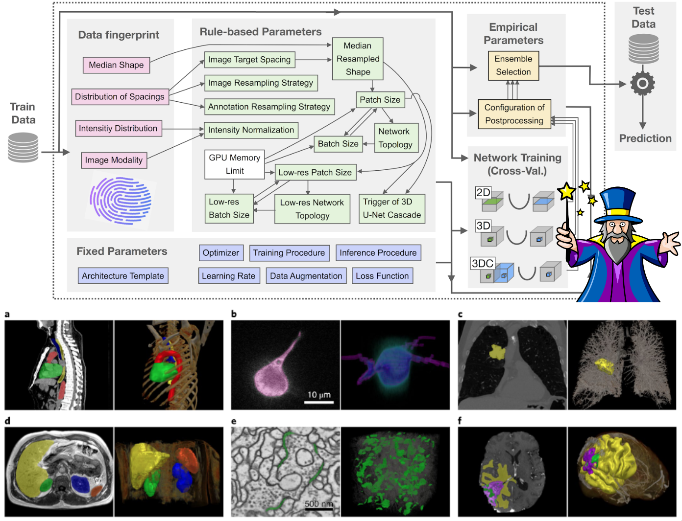
Figure: The nnU-Net pipeline automatically analyzes dataset properties ("fingerprint") and configures preprocessing, architecture, and training hyperparameters accordingly. Image adapted from Isensee et al., Nature Methods 2021.
8.6.1 The nnU-Net Philosophy
The core insight of nnU-Net is that methodology matters more than architecture. When you read a paper claiming a new architecture improves segmentation by 2-3%, consider: did they also tune the learning rate? The batch size? The data augmentation? The preprocessing? In most cases, these "boring" details have a larger impact than architectural novelty.
nnU-Net automates the entire pipeline configuration based on a "dataset fingerprint". These are properties like image dimensions, spacing, intensity distribution, and available GPU memory. This includes:
Preprocessing: Automatic resampling to handle anisotropic voxel spacing, intensity normalization based on modality (CT uses fixed HU windowing; MRI uses z-score per volume)
Architecture Selection: nnU-Net trains three configurations and ensembles the best:
- 2D U-Net: Processes slices independently (fast, works for any image size)
- 3D U-Net (full resolution): Processes 3D patches at native resolution
- 3D U-Net Cascade: First stage at low resolution for context, second stage at full resolution for detail
Patch & Batch Size: Automatically determined based on image dimensions and GPU memory. Larger patches provide more context; batch size is adjusted to fit memory.
Data Augmentation: Aggressive augmentation including rotation, scaling, elastic deformation, gamma correction, and mirroring—applied consistently across all experiments.
8.6.2 Results That Changed the Field
Without any manual tuning, nnU-Net achieved state-of-the-art or near state-of-the-art results on 23 public datasets spanning diverse modalities (CT, MRI, microscopy) and anatomical targets (brain, liver, cardiac, cellular). It won or placed highly in most major medical image segmentation challenges at the time of publication.
This was a wake-up call for the field: many "novel" architectures were not actually better than a properly-tuned baseline. The gains attributed to architectural changes were often confounded by differences in training setup.
8.6.3 Limitations
Despite its success, nnU-Net has important limitations:
Long Training Times: nnU-Net trains all three configurations (2D, 3D, cascade) and uses 5-fold cross-validation by default. A single dataset can take days to train, even on modern GPUs.
Not Memory Optimized: nnU-Net prioritizes segmentation accuracy over computational efficiency. It does not employ memory-saving techniques. Training 3D configurations often requires 11+ GB of VRAM, and inference on large volumes may require significant RAM.
Black-Box Decisions: While the automation is convenient, understanding why nnU-Net made certain choices (e.g., specific patch size, normalization scheme) requires digging through the generated configuration files. This can make debugging and customization challenging.
Less Flexibility: If you have domain-specific knowledge that could improve results (e.g., a custom loss function, architectural modification), incorporating it into nnU-Net requires modifying the codebase rather than simple configuration.
8.6.4 When to Use nnU-Net
nnU-Net is an excellent choice when:
- You need a strong baseline quickly
- You're working on a new dataset and don't know optimal hyperparameters
- Reproducibility is important (the automated pipeline eliminates human variability)
- You're benchmarking a new method and need a fair comparison
Consider alternatives when:
- Training time or computational resources are limited
- You need real-time inference or deployment on edge devices
- You have strong domain knowledge that should guide architectural choices
8.7 Segment Anything Model (SAM)
In section 8.3, we discussed how U-Net and its variants require training from scratch (or fine-tuning) for each specific segmentation task. Segment Anything Model (SAM) represents a fundamentally different approach: a foundation model pre-trained on an enormous dataset that can segment anything with minimal guidance.
8.7.1 What Makes SAM Different?
Unlike task-specific models like U-Net, SAM was trained on a dataset containing over 1 billion masks from 11 million images. This massive training allows SAM to:
- Segment without task-specific training - Point at an object, and SAM segments it
- Accept interactive prompts - Click points (positive or negative), draw bounding boxes, or provide rough masks
- Generalize across domains - Works on natural images, and with adaptation, medical images
8.7.2 SAM for Medical Imaging: Practical Applications
For medical imaging practitioners, SAM's primary value is as a rapid annotation tool. You can click a few points or draw a bounding box and get a rough segmentation that you can refine later.
8.7.3 Medical Variants
The original SAM was trained on natural images and struggles with medical imaging's unique characteristics (low contrast, unusual textures, 3D data). Several adaptations address this:
- MedSAM - Fine-tuned on 1.5 million medical image-mask pairs across 10+ modalities
- SAM-Med2D - Specifically adapted for 2D medical images
- SAM-Med3D - Extended to handle volumetric (3D) medical data
8.7.4 When to Use SAM vs Traditional Approaches
Choose SAM/MedSAM when:
- You need quick, interactive annotations
- You're bootstrapping a new dataset
- You want zero-shot segmentation without training
- You have diverse data and no task-specific model
Choose U-Net/nnU-Net when:
- You have labeled training data for your specific task
- You need fully automatic segmentation (no prompts)
- You require consistent, reproducible results
- You're deploying in a clinical pipeline
8.7.5 Try It Yourself
Meta provides an online demo where you can experiment with SAM's capabilities (just don't upload sensitive data to it!):
Demo: https://segment-anything.com/
For medical applications, consider starting with MedSAM:
Paper: Ma, J., et al. "Segment Anything in Medical Images." Nature Communications (2024)
Code: https://github.com/bowang-lab/MedSAM
Note: A deep understanding of SAM's architecture requires familiarity with Vision Transformers (ViT), attention mechanisms, and foundation model concepts. These topics are beyond the current tutorial's scope, but SAM remains a valuable practical tool even without understanding its internals.
References and Further Reading
Key Papers
- Ronneberger et al., "U-Net: Convolutional Networks for Biomedical Image Segmentation" (2015)
- Long et al., "Fully Convolutional Networks for Semantic Segmentation" (2015)
- Isensee et al., "nnU-Net: a self-configuring method for deep learning-based biomedical image segmentation" (2021)
- Kirillov et al., "Segment Anything" (2023)
Useful Libraries
- MONAI (Medical Open Network for AI)
- TorchIO (data loading and augmentation)
- nnU-Net framework
- Segment Anything